
Working Paper
WP 2016-339
How Well Does the Australian Aged Pension
Provide Social Insurance?
Emily Dabbs and Cagri Kumru
Project #: UM15-14
Regents of the University of Michigan
How Well Does the Australian Aged Pension
Provide Social Insurance?
Emily Dabbs
Research School of Economics, Australian National University
Cagri Kumru
Research School of Economics, Australian National University
November 2015
Michigan Retirement Research Center
University of Michigan
P.O. Box 1248
Ann Arbor, MI 48104
www.mrrc.isr.umich.edu
(734) 615-0422
Acknowledgements
The research reported herein was performed pursuant to a grant from the U.S. Social Security
Administration (SSA) funded as part of the Retirement Research Consortium through the University of
Michigan Retirement Research Center (5 RRC08098401-07). The opinions and conclusions expressed
are solely those of the author(s) and do not represent the opinions or policy of SSA or any agency of the
Federal Government. Neither the United States Government nor any agency thereof, nor any of their
employees, makes any warranty, express or implied, or assumes any legal liability or responsibility for the
accuracy, completeness, or usefulness of the contents of this report. Reference herein to any specific
commercial product, process or service by trade name, trademark, manufacturer, or otherwise does not
necessarily constitute or imply endorsement, recommendation or favoring by the United States
Government or any agency thereof.
Michael J. Behm, Gr
and Blanc; Mark J. Bernstein, Ann Arbor; Laurence B. Deitch, Bloomfield Hills; Shauna Ryder
Diggs, Grosse Pointe; Denise Ilitch, Bingham Farms; Andrea Fischer Newman, Ann Arbor; Andrew C. Richner,
Grosse Pointe Park; Katherine E. White, Ann Arbor; Mark S. Schlissel, ex officio
How Well Does the Australian Aged Pension
Provide Social Insurance?
Abstract
Social security plays an essential role in an economy, but if designed incorrectly can distort the
labor supply and savings behavior of individuals in the economy. We explore how well the
Australian means-tested pension system provides social insurance by calculating possible
welfare gains from changing the settings in the current means-tested pension system. This work
has been explored by other researchers both in Australia and in other pension-providing
economies. However, most research ignores the fact that welfare gains can be found by reducing
the cost of the program. To exclude these welfare costs, this paper fixes the cost of the system.
We find that the means-tested pension system is welfare reducing, but does provide a better
outcome than an equivalent-costing PAYG system. We also find that if the benefit amount is
held constant, and hence the cost of the pension program is allowed to vary, a taper rate of 1.0 is
optimal. However, once we fix this cost, a universal benefit scheme provides the best welfare
outcome.
Citation
Dabbs, Emily and Cagri Kumru. 2015. “How Well Does the Australian Aged Pension Provide
Social Insurance?” Ann Arbor, MI. University of Michigan Retirement Research Center
(MRRC) Working Paper, WP 2016-339.
http://www.mrrc.isr.umich.edu/publications/papers/pdf/wp339.pdf

1 Introduction
Social insurance plays an important role in the Australian economy, providing a form of insurance
to people against risks such as illness, disability and longevity. In the 2014-15 financial year ex-
penditure on social security and welfare is expected to account for over 30% of total government
expenditure, with assistance for the aged a key driver of expenditure growth.
1
Growth in expen-
diture on aged pension is a common theme across many countries, including the U.S., U.K. and
Europe. For this reason, the provision of aged pension is a topic of much debate, with government
policy experts and economists looking to reform current policies to ensure optimal provision of
benefits to elderly individuals in society.
The Pay As You Go (PAYG) system and the means-tested system are two pension programmes
analysed in the literature. PAYG is an intergenerational risk sharing system for social insurance
whereby agents pay a specific social insurance tax and are provided with a benefit in times of
retirement proportional to their average earnings. In times of a growing population and economic
growth, this system works well as the new generation is funding the retired generation. But where
an economy has an ageing population, with fewer working people funding more retirees, funding a
PAYG system starts to become problematic and raises the question of efficient benefit allocation.
Due to the funding problem a PAYG system faces, means-tested pension systems have been the
focus of many recent studies as this type of system reduces the fiscal burden through benefit target-
ing. This benefit targeting is achieved by providing payments to aged citizens based on their income
and savings. The means-tested system is currently employed in many countries, including Australia.
The focus of our research is to explore how changes to the Australian means-tested pension
system can provide welfare gains, using an open economy overlapping generations model. We first
compare the current system and a stylised PAYG system against an economy where no pension
system is in place, focusing on welfare gains and distributional effects. We then explore how changes
to the current means-tested pension settings impact the labour supply and savings behaviour of
individuals.
Possible welfare gains resulting from adjustments to social security systems have been explored
quite extensively. In the U.S. context, where a PAYG system is in place, Auerbach & Kotlikoff
(1987) find that the PAYG system significantly reduces welfare. However, their paper does not
take into account sources of uncertainty, which underlie the theory for government funded social
insurance. Huggett & Ventura (1999) and Imrohoroglu et. al (1995) extend on Auerbach and
Kotlikoff’s work by including life-span uncertainty and wage rate uncertainty. The results from
their work indicate that, in the presence of incomplete annuity markets, the U.S. PAYG system
can provide insurance benefits against longevity risk and income fluctuations.
Huggett & Parra (2010) take a different approach to assessing the U.S. social security system.
They first find the maximum welfare gains possible and then see how close the PAYG system and
variations of this system come to reaching the maximum welfare level. Their results are similar to
those found by Huggett & Ventura (1999) and Imrohoroglu et. al (1995), in that whilst the PAYG
1
This includes the following categories: Income support for seniors (age pension ), Residential and flexible care,
Veterans’ community care and support, Home support, Home care, National partnership payments - assistance to the
aged, Mature age income support, Allowances - concessions and services for seniors, Ageing and service improvement,
Workforce and quality, Access and information, and Other.
2
system doesn’t achieve the maximum welfare gains possible, it does provide significant welfare gains.
In recent years there has been a large amount of emerging literature on means-tested social
insurance systems. Sefton & van de Ven (2009) explored the U..K system with a means-tested
framework and found that means-tested benefits are strictly preferred to a universal benefit struc-
ture. However, they also found that the means-tested system provides a disincentive for richer
households to save but encouraged savings in poorer households. Kumru & Piggott (2009) ex-
tended this work further by incorporating a second tier of the U.K. system, which represents a
PAYG system, and explore optimal taper rates. They also find that a means-tested system is
preferred to a universal pension system, and further, that a 100% income taper rate provides the
highest level of welfare gains.
In the Australian context, Kudrna & Woodland (2011) explore the impacts of different income
taper rates on the savings and work behaviour of Australians and find, similar to Sefton & van de
Ven’s (2009) results, that the current system provides a disincentive for older middle and higher
income Australians to work. Tran & Woodland (2014) extend on this work by exploring both
changes to income taper rates and benefit payment rates. They find that, conditional on compul-
sory pension systems, when the maximum pension benefit is relatively low, an increase in the taper
rate will always lead to a welfare gain. However, when maximum pension benefits are relatively
more generous an increase in the benefit and taper rate will lead to welfare declines.
This paper builds on previous work, notably Kumru & Piggott (2009), by adjusting both income
taper rates and benefit payments simultaneously to fix the present value cost of the pension benefit
system. This allows us to exclude welfare gains due solely to reduction in the cost of the system,
and focus on identifying welfare gains due to reallocation between individuals.
We find that, similar to Auerbach & Kotlikoff (1987) and Tran & Woodland (2014), the means-
tested system is welfare reducing. However, it provides higher welfare outcomes when compared
to a PAYG style system. Significant differences in savings behaviour can be seen between poor
and wealthy households under each system, with means-tested providing a disincentive for wealthy
households to save. We also find that, similar to findings by Trans & Woodland, the largest wel-
fare gains within the means-tested system can be made with a taper rate of 1.0 as the insurance
incentive offsets the distortionary effects on savings. However, when we fix the cost of the system
a universal benefit scheme provides the optimal outcome. This implies that when the cost of the
system is allowed to vary, welfare gains are due to a lower costing system.
The paper is organised as follows. Section 2 outlines the model that will be used in the anal-
ysis. Section 3 discusses the parameterization of the model to the Australian economy. Results
are presented in section 4 with a sensitivity analysis presented in section 5, and section 6 concludes.
This section provides detail on the model used to
analyse changes to the Australian pension pro-
gramme. We use a simple partial equilibrium economy comprised of heterogeneous households, a
production sector and a government sector.
3
2 The Model

µ
j−1
v
j
µ
j
= for j = 2, 3, 4, ...J
1 + n
1−ρ
c (1 − l)
1−ϕ
u(c, 1 − l) = + κ
1 − ρ 1 − ϕ
2.1 Demographics and Endowments
Our model economy is populated by overlapping generations who live up to a maximum of J peri-
ods, with conditional probability of surviving from age j to j + 1 denoted by v
j
. Every period t a
new generation is born with the population growing at an exogenous rate n.
2
There are constant
cohort shares due to the constant growth rate and stationary demographics, which are defined as:
(1)
J
j=1
µ
j
= 1 with
Individuals face exogenous age-efficiency profiles,
j
, which represent changes to ability over
time and are the same for all individuals. The productivity of an individual at a particular time
period depends on not only on their age j, but they are also faced with idiosyncratic wage rate
shocks s
j
.
2.2 Preferences
In our model all individuals have identical preferences over consumption and leisure, which is de-
noted by the expected utility function with discount factor β as follows:
J
j
E
β
j
v
i
u(c
j
, 1 − l
j
)
j=1 i=1
(2)
Each period individuals are endowed with 1 unit of
labour, and they choose the amount of
labour and leisure in that period, given by l
j
and 1 − l
j
respectively. Instantaneous utility is ob-
tained through consumption and leisure, and defined as:
(3)
The coefficient of relative risk aversion is
given by ρ ∈ (0, +∞) with the the inter-temporal
elasticity of substitution of consumption given by
1
ρ
. The Frisch elasticity of leisure is given by −
ϕ
1
,
with ϕ ∈ (0, +∞). κ captures the dislike for work relative to enjoyment of consumption.
2.3 Production sector
The production sector consists of many perfectly competitive large firms, which is equivalent to
one large firm that maximises profits. The representative firm produces output Y at time t using
effective labour services L and capital K with exogenously given technology level A. The technology
is represented by a Cobb-Douglas constant returns to scale production function:
L
1−α
Y
t
= A
t
K
α
t
t
(4)
2
The time notation is excluded from the rest of the model description for simplicity.
4
The firm chooses capital and labour to maximise its profits, which can be expressed as:
max
K,L
{AK
α
L
1−α
− rK − wL} (5)
2.4 Government sector
The government runs a pension programme and makes consumption expenditure. This section
outlines the two pension programmes used in this model, as well as the taxation on consumption
and income.
Taxation
The government collects tax on both income and consumption to finance its general expenditure
and age pension. The consumption tax is set at rate τ
c
. Australia’s income taxation system is
progressive, whereby individuals in higher income bands are taxed more than those in lower income
bands. It can be expressed as:
T (y
j
) = T
k
+ τ
k
(y
j
− ¯ y
j
∈ [ ¯ y
k
¯
+1
] y
k
), y
k
, (6)
where τ
k
is the marginal tax rate, T
k
is the flat tax and y¯
k
is the income threshold for the
income bucket k. In the Australian context we have T
1
= 0, τ
1
= 0 and T
k
y
k
−= T
k−1
+ τ
k
( ¯ y
k
¯
−1
).
Means-tested pension
In the Australian benchmark model, the government runs a means-tested pension system. The
benefit amount b(y
j
, a
j
) is subject to two tests, an income test and an asset test, and can be written
as:
b
m
(y
j
, a
j
) = min{b
y
(y
j
), b
a
(a
j
)} (7)
where b
y
(y
j
) is the income test pension and b
a
(a
j
) is the asset test pension. So an individual
receives the minimum of the two tests. Each test is subject to a threshold amount and is given by:
b
y
(y
j
) =
b
max
if y
j
≤ ¯y
1
b
max
− t
y
(y
j
− ¯y
1
) if ¯y
2
< y
j
< ¯y
2
0 if y
j
≥ ¯y
2
(8)
y
1
+ b
max
/t
y
y¯
2
= ¯where y¯
1
and are the income thresholds and t
y
is the taper rate for income,
which is the rate at which the benefit is reduced for each dollar over y¯
1
.
b
max
if a
j
≤ a¯
1
b
max
− t
a
(a
j
− a¯
1
) if a¯
2
< a
j
< a¯
2
b
a
(a
j
) =
0 if a
j
≥ a¯
2
(9)
5
a
1
+ b
max
/t
a
a¯
2
= ¯where a¯
1
and are the asset thresholds and t
a
is the taper rate for assets,
which is the rate at which the benefit is reduced for each dollar over a¯
1
.
Pay-as-you-go (PAYG) pension
The PAYG pension system collects a specific social security tax from workers during their work
life, and then provides a payment that is proportional to the individuals average earnings. In this
system, the social security tax rate is denoted τ
ss
and the tax collected through the social security
tax can be expressed as:
T
s
= min
j
τ
ss
l
j
j
s
j
w
e
max
(10)
where e
max
is the maximum taxable level.
x
s
The benefit provided to retirees is denoted b
s
(x
s
) where is an accounting variable, i.e. equally
weighted earnings before retirement.
2.5 An Individual’s Decision Problem
Individuals are heterogeneous with respect to state variables of age, working ability and asset hold-
ings. An individual’s state variables at age j are denoted by x
j
= (e
j
, a
j
). Individuals realise their
state x
j
and choose the optimal consumption c
j
, leisure time 1 − l
j
(or working time l
j
) and end
of period asset holdings a
j+1
given wage and interest rates, government tax and pension policies,
survival probabilities, and their working ability.
Individuals have three sources of income; returns from savings ra
j
, effective labour earnings
l
j
j
s
j
w, and possible pension payment b
j
. Therefore their income can be expressed as:
y
j
=
ra
j
+ l
j
j
s
j
w if j < j∗
ra
j
+ b
j
(x) if j ≥ j∗
From this we can express an individual’s growth-adjusted budget constraint as:
c
j
+ (1 + g)a
j+1
≤ (1 + r)a
j
+ (1 − τ
s
− τ
p
)l
j
j
s
j
w − τ(y
i
) when j < j∗
c
j
+ (1 + g)a
j+1
≤ (1 + r)a
j
+ b
j
+ b
'
j
(x) − τ (y
i
) when j ≥ j∗
c
j
≤ (1 + r)a
j
+ b
j
(x) + b
'
j
(x) − τ (y
i
) when j = J
(11)
and we assume that individuals cannot borrow against future income:
a
j
≥ 0, ∀j (12)
6
J
K = µ
j
a
j
(x)dΛ
j
X
j=1
J
L = µ
j
l
j
(x)dΛ
j
X
j=1
J
C = µ
j
c
j
(x)dΛ
j
X
j=1
Hence, an individual’s decision problem in our model can be written as the dynamic program-
ming problem below, where V
j
is the value function of the individual at age j and x
'
is the next
period state vector.
V
j
(x) = max {u(c
j
, l
j
) + βv
j+1
EV
j+1
(x
'
)}
c
j
,l
j
(13)
subject to equations 11 and 12.
2.6 Equilibrium
Our equilibrium definition follows Auerbach & Kotlikoff (1987), Imrohoroglu et. al (1995), and
Kumru & Piggott (2009).
Given government policy settings for taxation and the pension system, the constant population
growth rate, and exogenous interest rate, a stationary equilibrium is such that:
1. a collection of individuals’ decisions {c
j
(·), l
j
(·), a
j+1
(·)}
J
j=1
solve the individual decision prob-
lem (13) subject to constraints (11) and (12)
2. age dependent distributions of individuals are calculated as:
Λ
j+1
(x) = (s
j+1
, s
j
) dΛ
j
s
X
(s
j+1
, s
j
) where is the transition matrix for the shocks. Λ
1
(x) is given.
3. the firm chooses labour and capital inputs to solve the maximisation problem (5)
4. the lump-sum bequest transfer (Ω) is equal to the sum of accidental bequests:
J
Ω = µ
j
(1 − v
j+1
(z))a
j
(x)dΛ
j
X
j=1
5. aggregate capital (K), labour (L) and consumption (C) is derived from individuals’ behaviour
7

J
j∗−1
µ
j
b
m
(x)dΛ
j
= τ
m
µ
j
y
j
(x)dΛ
j
X X
j=j∗ j=1
J
j∗−1
b
ss
(x)dΛ
j
= τ
ss
µ
j
µ
j
min{y
j
(x), y
max
}dΛ
j
X X
j=j∗ j=1
3 Calibration
6. age pension programmes are self-financing:
7. the Government budget constraint is satisfied at every period:
T
inc
+ Ω + τ
c
C+ = G
8. goods market clears:
C + (1 + g)(1 + n)K + G = Y + (1 − δ)K
This section details the parameters used in our model. We calibrate the benchmark model to the
Australian economy. The key parameters are detailed in Table 1.
Table 1: Parameters
Parameters Model Observation / Comment / Source
Demographics
Initial age j = 1 Age 21
Maximum age j = 65 Age 85
Retirement age j∗ = 55 Age 65
Annual Population Growth n = 0.012 ABS data
Survival probabilities
Age efficiency profile
v
j
j
ABS data
HILDA data
Preferences
Annual discount factor β = 0.99 Match Australian saving behaviour
Risk adversion parameter ρ = 2 Tran & Woodland (2011)
Frisch elasticity γ = 0.35 Buddelmeyer et. al (2007)
Production
Capital share of GDP α = 0.4 Tran & Woodland (2014)
Interest rate r = 0.0495 Average10 year Treasury bond
Government
Government consumption
Consumption tax
G = 0.14
τ
c
Tran & Woodland (2014)
Endogenously determined
Income taxes
Means-tested pension
PAYG pension
τ
j
, T
j
, ¯y
j
b
max
, t
y
, t
a
, ¯y
1
, ¯a
1
2014-15 tax schedules
2014-15 pension rules
Huggett & Parra (2010)
Demographics
Our model assumes individuals are born, or become economically active, at age 21 (j = 1) and
live up to a maximum age of 85 (j = 65). The population growth rate is set to 1.2% which is the
8

Australian average over the last 10 years. The conditional survival probabilities (v
j
) of individuals
are estimated using ABS data on death rates.
The age efficiency profiles (
j
) correspond to hourly wage rates by age. We have estimated the
Australian age efficiency profile using the data from the Household, Income and Labour Dynamics
in Australia (HILDA) survey
3
, similar to Tran & Woodland (2014).
We estimate the idiosyncratic wage rate shocks using a five-point discrete Markov chain process
as described by Tauchen & Hussey (1991). Similar to Cho & Sane (2011) we use the Gini coefficient
as a measure of the variance, which is 0.34 taken from Greenville et. al. (2013). The shocks are
calculated as s
k
= {0.2069, 0.4133, 0.7721, 1.4424, 2.8819} and the probabilities for each shock are
calculated as p
k
= {0.0988, 0.2418, 0.3188, 0.2418, 0.0988}
Preferences
We set ρ = 2 which is a standard assumption for Australia. We then set κ = 1 to normalise to
unity. We calibrate ϕ to match the Frisch elasticity of γ = 0.35. We use β = 0.99 to match the
Australian savings behaviour, which is also used by Tran & Woodland (2014).
Production sector
We use the capital share of GDP α = 0.4 as calculated in Tran & Woodland (2014). As Australia
is a small economy, we use a partial equilibrium model where factor prices are set exogenously. We
set the interest rate r = 0.0495 which is the average of Australian Treasury bonds over the last 10
years.
Government sector
Figure 1: Marginal Tax Rates
The consumption tax rate adjusted endogenously within the model to ensure the government
budget is balanced. We use a quadratic function to approximate the marginal tax rates individuals
3
HILDA is a longitudinal household survey that collects data on income, work, and family / household formation.
Similar to Tran & Woodland (2011) we use data from the first 7 waves of the survey for our age efficiency profiles.
9

face, similar to that used by Kumru & Piggott (2009) and Huggett & Parra (2010). The actual
marginal tax rates versus the estimated marginal tax rates are shown in Figure 1, which verifies
that the quadratic function matches real marginal tax rates fairly closely.
We use the means-tested pension rates as detailed by the Department of Human Services for
2014-15. This includes a taper rate on income of t
y
= 0.5, a benefit reduction rate on assets of
t
a
= 0.0015, an income threshold of y¯
1
= $4, 160 per year, an asset threshold of a¯
1
= $348, 500 and
a benefit payment of $14, 846 per year. As our model does not adequately capture homeownership,
we use the asset threshold for individuals who do not have a family home.
To compare the Australian means-tested pension system to a PAYG system, we use Huggett
& Parra (2010) benefit payment parameters for the PAYG system. This is expressed as a benefit
payment function in Figure 2. We set the social security tax such that the net present value of the
system matches the benchmark Australian means-tested system, in this case τ
ss
= 21.8%.
Figure 2: PAYG Benefit Function
4 Simulation Results
This section first compares our benchmark model to the current Australian economy before explor-
ing different policy changes. When discussing policy changes we focus on comparing means-tested
pension system and PAYG pension systems before considering changes to taper rates and pension
payment rates, holding the cost of the programme constant.
4.1 Benchmark Model
Before considering changes to the Australian means-tested pension system, we first examine key
outputs of our model to see that it matches features of the Australian economy.
10
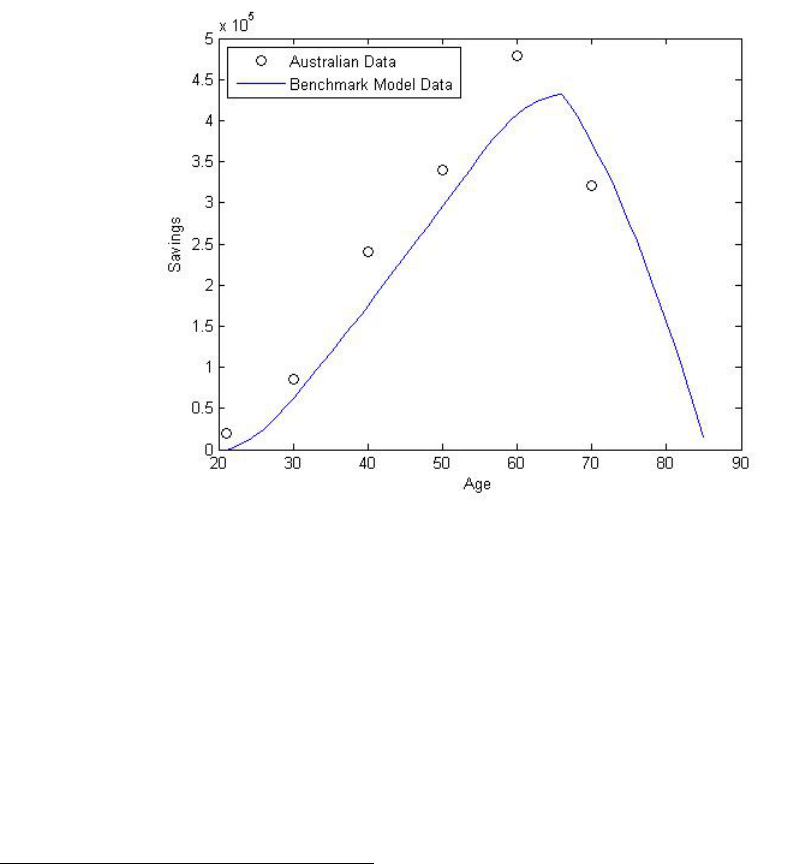
Asset profile
4
In order to compare our model output to real Australian data, we use the HILDA survey results
on assets and wealth distribution. As can be seen in Figure 3, our model generates the same life-
cycle asset accumulation whereby individuals accumulate assets early in their life before drawing
down on them during retirement. We can see that assets are lower earlier in life, starting at 0 when
j = 1, as we constrain our model such that individuals start their working life with no assets. We
can also see that peak savings, while at the same stage of life in both sets of data, is much higher
in the real data compared to our model output. Housing is often cited as a key incentive for saving
in the Australian context, and while excluded from the data there may be flow on to other savings
behaviour. So this difference in peak savings may be attributed to the fact that our model doesn’t
include housing.
Figure 3: Asset Profile
Labour market
Our model matches the life cycle labour supply behaviour of individuals fairly well, as shown
in Figure 4. A notable difference being that younger individuals work more than the observed data
shows. This is primarily due to the assumption in our model that individuals enter their working
life with no assets and cannot borrow. We also make the retirement decision exogenous in our
modeling, meaning that individuals leave the workforce at 65.
4.2 Comparison of Pension Systems
In this section we compare the benchmark model and a stylised PAYG pension system with the
Australian economy without a pension system in place. We focus on welfare differences and explore
4
Assets in our model do not include compulsory superannuation or housing
11

∗
V (x
0
)
EV =
∗
− 1
V (x )
1
1/(1−ρ)
,
Figure 4: Labour Profile
changes in savings and labour supply behaviour.
A pension system has two opposing impacts on individuals behaviour; it provides a form of
risk-sharing but also distorts individuals labour supply and savings behaviour. We use the results
in Table 2 to assess which of these is the dominant force in the PAYG pension system, means-tested
pension system and an economy without a pension system.
To compare the models in terms of welfare we compute the consumption equivalent varia-
tion (CEV), which is a standard method following on from Conesa et. al (2009) and Kumru &
Thanopoulos (2011)
5
. We use the model with no pension as the baseline for analysis in this section,
meaning a positive CEV indicates a welfare gain compared to the model with no pension and a
negative CEV indicates a welfare loss compared to the model with no pension. We also use the
model with no pension as the baseline model for comparing relative changes in savings and labour
supply.
Table 2: Results from Comparison of Pension Systems
System Cost of Pension System CEV (%) Aggregate Labour Aggregate Savings
No pension NA 0 100 100
PAYG -1.54 -23 117.2 60.1
Means-tested -1.54 -22 116.5 61.1
As shown in Table 2, both pension systems are welfare reducing. Individuals in both the means-
5
As described in Kumru & Thanpoulos (2011) C where x
∗
0
is the benchmark model
allocation and x
∗
1
is the new system allocation
12

tested and PAYG system have much lower savings over their life-span than under the model with no
pension system. This aligns with the results from Tran & Woodland (2014), Auerbach & Kotlikoff
(1987), and Imrohoroglu et. al (1995), which consistently find that pension systems are welfare
reducing due to the dominant effect of incentive distortion. Figure 5 shows this distortion clearly
through the savings behaviour of individuals under each of the systems.
Figure 5: Average Asset Profiles
Now we take a closer look at the differences between the two pension systems. As can be seen
from Table 2, a PAYG system has a lower CEV (-23%) when compared to a means-tested system
(-22%). This provides an additional layer of analysis to show that the averse incentive effects are
marginally smaller under the means-tested system compared with the PAYG system. To fully un-
derstand the differences between the two systems, we compare the different impacts on the poor
and wealthy in the economy.
Let us first consider the lowest earners in the system, and examine their savings and labour
supply behaviour. As can be seen by Figure 6, lowest earners do not change their savings or labour
supply behaviour between the two systems. This is because they have no incentive to lower savings
under a means-tested system, given they are already receiving the largest benefit. In the case
of a PAYG system, they cannot increase their labour supply sufficiently to increase their benefit
payment in retirement, hence they have lower utility under a PAYG system.
We can see in Figure 7 that the highest earners accumulate assets earlier in life in a PAYG sys-
tem, reaching a much higher peak of savings than under a means-tested system. The disincentive
to save under a means-tested system for wealthy individuals is due to the fact that their benefit in
retirement reduces if their savings levels are too high. There is no such disincentive under a PAYG
system, hence the higher savings and higher utility for wealthy individuals in a PAYG system.
13

Figure 6: Labour Supply and Savings Behaviour of Lowest Earners
Figure 7: Labour Supply and Savings Behaviour of Highest Earners
We conclude that while the means-tested pension system is welfare reducing, the reduction in
welfare is lower than that under the PAYG pension system. The two systems have very different
impacts on the savings behaviour of individuals, with the means-tested system providing a disin-
centive for wealthier individuals to save.
4.3 Changes to Means-tested Policy
In this section we explore changes to the income taper rate in the means-tested system. By varying
the taper rate we are changing the effective marginal tax on income in retirement, with a higher
taper rate increasing the effective marginal tax. Given savings are the single source of income in
retirements, by changing the taper rate we expect to see changes to savings behaviour. We first
explore these effects in a model with varying cost, before examining how imposing constant cost
of the programme changes the results. In this section we use the benchmark model as the baseline
for examining welfare gains with CEV and relative changes to savings and labour.
Variable system cost
We first simulate a numb
er of
alternative model economies where we vary the taper rate in the
means-tested pension holding the income threshold, benefit payment, and asset testing constant.
A different taper rate has two main effects; it changes the value of the benefit paid to retirees and
simultaneously changes the number of retirees who receive benefit payments. Table 3 reports the
welfare effects as well as the main aggregate variables we are interested in.
The results reported in Table 3 indicate that in our model economy a taper rate of 1.0 provides
14

Table 3: Results from Changes to the Taper Rate
Taper Rate Maximum Benefit Cost of Pension System CEV Savings Labour
0.0 15,000 -1.94 -7.550 92.4 98.8
0.1 15,000 -1.85 -4.429 96.1 101.1
0.2 15,000 -1.78 -3.027 97.7 100.7
0.3 15,000 -1.71 -3.004 96.8 100.8
0.4 15,000 -1.63 0.390 100.9 99.9
0.5 15,000 -1.54 0.000 100.0 100.0
0.6 15,000 -1.44 4.091 104.8 99.0
0.7 15,000 -1.38 5.130 105.9 98.7
0.8 15,000 -1.29 7.325 108.5 98.2
0.9 15,000 -1.22 8.599 109.6 97.9
1.0 15,000 -1.17 9.597 110.6 97.7
the greatest welfare gain, similar to the conclusion from Kumru & Piggott (2009) and Tran &
Woodland (2014). At this taper rate, we are maximising the risk-sharing mechanism while min-
imising the distortionary impact on savings behaviour.
We can see the distortionary effects on savings increase as the taper rate decreases due to fact
that individuals have a lower incentive to save for their retirement. As the taper rate decreases,
more individuals become eligible for the pension programme, meaning they do not need to save as
much for their retirement. Under a universal benefit (taper rate = 0.0), everyone receives a benefit
regardless of their income, meaning even the wealthiest individuals in the economy can reduce their
savings and still maintain their consumption in retirement.
The impact on labour supply behaviour is much less significant, with a lower taper rate resulting
in higher labour supply behaviour. Again, this result is due to the fact that a higher taper rate
results in more individuals lowering their labour, and hence savings and income in retirement, to
ensure their eligibility for the pension system.
The results in Table 3 show that the cost of the system increases as the taper rate decreases,
as individuals who received very little or no pension benefit now receive a higher payment. This
means our results cannot indicate if the welfare gains due to higher taper rates are due to an opti-
mal distribution of benefits or simply due to a lower costing pension programme. To explore this
further, we fix the cost of the programme by varying the benefit amount, and compare the changes
in welfare and savings behaviour.
Constant system cost
We now simulate a number of alternative model economies where we vary the taper rate and
benefit amount in the means-tested pension, holding the cost of the programme constant. Again
we hold the income threshold and asset testing constant. By keeping the cost of the programme
constant we can ensure that changes in welfare are solely attributed to the distribution of benefit
payments in the economy and exclude any welfare changes due to a change in the cost of the pension
system.
The results in Table 4 show that when the cost of the system is held constant, the optimal
15

5 Sensitivity Analysis
Table 4: Results from Changes to the Taper Rate with Constant Cost
Taper Rate Maximum Benefit Cost of Pension System CEV Savings Labour
0.0 9,000 -1.54 0.697 100.6 99.8
0.1 10,000 -1.54 0.496 100.2 99.9
0.2 12,000 -1.54 0.483 100.1 99.9
0.3 13,000 -1.54 0.363 100.1 99.9
0.4 14,000 -1.54 0.183 99.8 100.0
0.5 15,000 -1.54 0.000 100.0 100.0
0.6 16,000 -1.54 -0.007 100.0 100.0
0.7 17,000 -1.54 -0.096 99.9 100.1
0.8 17,000 -1.54 -0.126 99.8 100.1
0.9 18,000 -1.54 -0.191 99.7 100.1
1.0 19,000 -1.54 -0.292 99.6 100.1
taper rate is 0.0, a universal benefit scheme. This directly opposes the results from the variable
cost system, indicating that the driver for welfare gains under a variable cost pension programme
is lower cost, and hence lower tax on individuals.
Under the fixed cost economies, changes in the taper rate also produce opposing results for sav-
ings and labour supply behaviour. As the taper rate and benefit payment increase, the incentive
to lower savings increases as individuals reduce their income in retirement to become eligible for
the pension programme.
From this analysis, we conclude that under a system with a fixed benefit, a taper rate of 1.0 is
preferred to all other taper rates. Lower taper rates distort the savings behaviour of individuals in
the economy through the higher tax rate needed to fund the pension programme. However, when
we hold the cost of the system the same, we find that a universal benefit is preferred. As the benefit
payment is lower, the distortionay effects on savings behaviour are minimised. This is an important
result as it highlights that the distortionary effects of changes to taper rates within a means-tested
pension system are due to changes in tax rates on individuals. Changes to the taper rate under a
fixed cost pension system produce the opposite affect, with a universal benefit providing the best
welfare outcome. Again, this indicates that the results from a variable cost pension programme are
driven by the cost of the system, rather than the distribution of benefits.
In this section we analyse how changes to parameters in the
model impacts the results. This
provides evidence that our results are robust. We consider these changes to parameters; survival
probabilities, age efficiencies, and risk aversion. Within our analysis we focus on our key findings
from Section 4.3; optimal taper rates under fixed and variable cost pension systems.
16

5.1 Survival Probabilities
We consider the current Australian survival probabilities and lower survival probabilities
6
as pic-
tured in Figure 8, and explore how changes to these probabilities impact our findings.
Figure 8: Conditional Survival Probabilities
Table 5: Survival Probabilities with Changing Taper Rates
Taper Rate
Variable cost
CEV (%)
High survival rates
Savings Labour CEV (%)
Low survival rates
Savings Labour
0.0 -7.550 92.4 98.8 -5.286 96.0 101.5
0.25 -1.969 98.5 100.4 -3.724 96.8 101.0
0.5 0.000 100.0 100.0 0.000 100.0 100.0
0.75 6.661 107.4 98.3 3.891 103.3 98.9
1.0 9.597 110.6 97.7 7.652 106.5 97.9
Fixed cost
0.0 0.697 100.6 99.8 0.866 100.4 99.8
0.25 0.338 100.0 100.0 0.422 100.4 99.9
0.5 0.000 100.0 100.0 0.000 100.0 100.0
0.75 -0.083 99.8 100.1 -0.101 99.9 100.0
1.0 -0.292 99.6 100.1 -0.258 99.9 100.1
We can see from our results in Table 5 that survival probabilities have an impact on savings
behaviour and welfare under a means-tested pension system. However, the results align with our
findings in Section 4 in that a taper rate of 1.0 produces the largest welfare gain in a variable cost
model due to lower tax rates. Under a fixed cost model we can see that a universal benefit provides
the best welfare outcome, which aligns with our results from Section 4.3.
6
For the lower survival probabilities we use U.S. values as used by Huggett & Parra (2010)
17
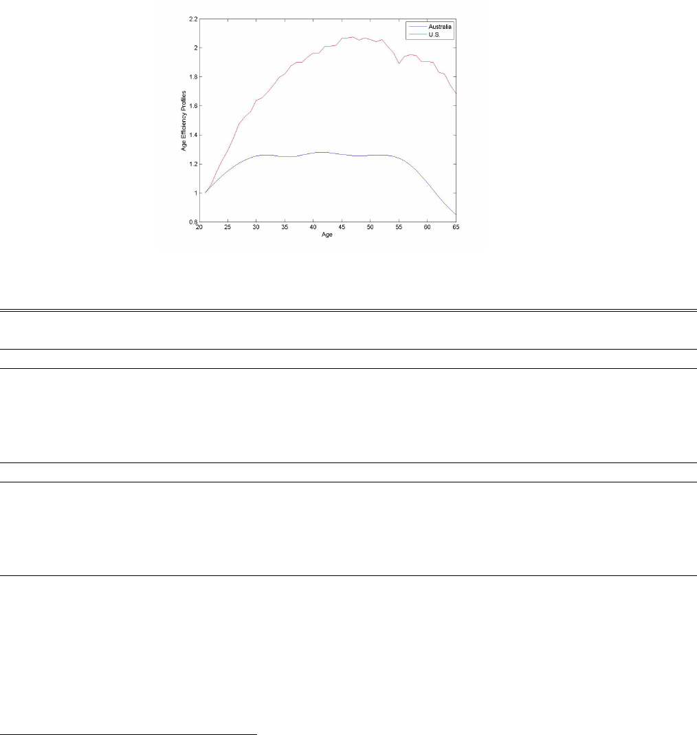
5.2 Age Efficiency Profiles
We consider the current flat efficiency profile used in Australia and a more concave age efficiency
profile
7
shown in Figure 9. We examine if the distribution of age efficiency impact our findings,
focusing on how larger differences in potential earnings across age groups impact welfare and savings.
Figure 9: Age Efficiency Profile
Table 6: Age Efficiencies with Changing Taper Rates
Flat distribution
Savings
Concave distribution.
Savings Taper Rate CEV (%) Labour CEV (%) Labour
Variable cost
0.0 -7.550 92.4 98.8 -7.215 92.8 102.1
0.25 -1.969 98.5 100.4 -3.847 95.7 101.1
0.5 0.000 100.0 100.0 0.000 100.0 100.0
0.75 6.661 107.4 98.3 2.140 99.9 99.5
1.0 9.597 110.6 97.7 3.383 101.4 99.1
Fixed cost
0.0 0.697 100.6 99.8 0.630 100.8 99.8
(%) 0.25
0.5
0.338
0.000
100.0
100.0
100.0
100.0
0.178
0.000
100.2
100.0
99.9
100.0
0.75 -0.083 99.8 100.1 -0.201 99.9 100.1
1.0 -0.292 99.6 100.1 -0.525 99.8 100.2
Table 6 results show that under a variable cost programme with a concave distribution of age
efficiencies, a taper rate of 1.0 produces the largest welfare gain. This result aligns with our conclu-
sion in Section 4, indicating that while the distribution of age efficiencies will impact the magnitude
of the welfare gain, it will not change the directional impact a change in the taper rate produces.
We can also see from Table 6, that the welfare gains from changing taper rates under a variable
cost programme with a concave distribution of age efficiencies are optimised for a universal benefit
7
For the concave age efficiency profile we use data on the U.S. as reported by Huggett & Parra (2010)
18

6 Conclusion
under a fixed cost model. Again, this is due to the fact that the welfare gains under from increasing
taper rates under a variable cost programme are due to lower tax, not better distribution of benefits.
We conclude that while different age efficiency profiles do impact the size of the welfare gain
and changes in individuals labour supply behaviour under different taper rates within a means-
tested pension system, the results are similar to those in Section 4. Our results come to the same
conclusion as Section 4, that welfare gains under a variable cost programme are not present under
a fixed cost model.
5.3 Risk Aversion
In this section we use a higher risk aversion parameter of 3 and explore whether this impacts our
results. A higher risk aversion parameter is representative of a more risk averse economy.
Table 7: Risk Aversion with Changing Taper Rates
Taper Rate Benefit Cost CEV (%) Savings Labour
Variable cost
0.0 15,000 -2.07 -8.433 94.3 102.1
0.25 15,000 -1.91 -3.982 97.4 101.0
0.5 15,000 -1.65 0.000 100.0 100.0
0.75 15,000 -1.38 6.445 105.1 98.65
1.0 15,000 -1.22 15.548 111.5 96.8
Fixed cost
0.0 9,000 -1.65 0.915 100.6 99.8
0.25 12,000 -1.65 0.395 100.2 99.9
0.5 15,000 -1.65 0.000 100.0 100.0
0.75 16,000 -1.65 -0.154 100.0 100.0
1.0 18,000 -1.65 -0.551 99.6 100.2
Table 7 illustrates that in an economy with a higher risk aversion
parameter, the results from
Section 4 still hold; a taper rate of 1.0 maximises welfare under a variable cost pension system and
a universal benefit maximises welfare under a fixed cost system.
Pension programmes play an important role in society b
y providing insurance against longevity
risk. However, these pension programmes can distort labour supply and savings behaviour of indi-
viduals, resulting in welfare losses. In this paper we explore how changes to the current Australian
pension system impact welfare.
The design of pension systems is a topic of many recent studies given their role in society. Our
work builds on that by Kumru & Piggott (2009), using an overlapping-generations model to explore
changes in savings and labour behaviour in response to changes in the means-tested taper rate. We
also examine welfare differences between an economy with no pension system, and that with either
19
a PAYG system or means-tested system.
Previous research has focused on changes to taper rates within the means-tested pension pro-
gramme and the resulting change in welfare. However, there has been little consideration to how
the change in the programme cost interplays with the change in welfare. Our work extends on the
current body of research by changing both the taper rate and benefit payment to hold the cost of
the programme constant, and then considering the impact on welfare.
We find, similar to Auerbach & Kotlikoff (1987) and Tran & Woodland (2011), that a means-
tested system is welfare reducing. However, a means-tested system does provide a welfare gain
compared to a similar costing PAYG system. We also find that, similar to previous work by Kumru
& Piggott (2009) and Tran & Woodland (2011), a taper rate of 1.0 provides the best welfare out-
come in a pension system with fixed benefit and variable cost. However, when we hold the cost of
the programme constant, we find an opposing impact on welfare, with a universal benefit providing
the maximum welfare. This is due to the fact that under a variable cost system lower taper rates
result in higher costs, and these costs are financed through taxation of individuals during their
working life which drives the welfare losses. Once the cost for the system is held constant, we see
that lower benefits paid to all individuals provides the best welfare outcome.
Our model assumes evenly distributed income through the wage rate shocks. Given the results
from our sensitivity analysis on age efficiency profiles, we would suggest that exploration of varying
shock distribution would provide an interesting extension on our work. We also consider inclusion
of superannuation and endogenous retirement decision would be beneficial in future research. Fi-
nally, our model assumes constant population age distribution. Give that there is growing pressure
on government financing of aged pension from an ageing population, inclusion of this phenomenon
would provide an interesting extension to our work.
20
References
[1] Auerbach, A. J., & Kotlikoff, L. J. 1987. Dynamic Fiscal Policy. New York, NY, USA: Cam-
bridge University Press.
[2] Buddelmeyer, H., Lee, W. S., Wooden, M. & Vu, H. 2007. Low Pay Dynamics: Do Low-
Paid Jobs Lead to Increased Earnings and Lower Welfare Dependency Over Time. Melbourne
Institute of Applied Economic and Social Research
[3] Cho, S.W., & Sane, R. 2011. Means-tested Age Pension and Homeownership: Is There a Link?
Macroeconomic Dynamics, 17, 1281 - 1310.
[4] Conesa, J. C., Kitao, S., Krueger, D. 2009. Taxing capital? Not a bad idea after all!. American
Economic Review 99, 25-48.
[5] Greenville, J., Pobke, C., & Rogers, N. 2013. Trends in the Distribution of Income in Australia.
Productivity Commission Staff Working Paper
[6] Hockey J.B. Cormann, M., Budget Strategy and Outlook: Budget Paper No. 1, Budget 2014-
15, Commonwealth of Australia, Canberra
[7] Huggett, M., & Ventura, G. 1999. On the distributional effects of social security reform. Review
of Economic Dynamics, 2, 498-531.
[8] Huggett, M., & Parra, J. C. 2010. How Well Does the U.S. Social Insurance System Provide
Social Insurance? Journal of Political Economy, 1, 76-112.
[9] Imrohoroglu, A., Imrohoroglu, S., & Joines, D. H. 1995. A life cycly analysis of social security.
Economic Theory, 6, 83-114.
[10] King, R. G., Plosser, C. I., & Rebelo, S. 2002. Production, Growth, and Business Cycles:
Technical Appendix. Computational Economics, 20, 87-116.
[11] Kudrna, G., & Woodland, A. 2011. An Intertemporal General Equilibrium Analysis of the
Australian Age Pension Means Test. Journal of Macroeconomics 33, 61-79.
[12] Kumru, C., & Piggott, J. 2009. Should Public Retirement Provision Be Means-tested? ABS
Research Paper No. 2009 AIPAR 01.
[13] Kumru, C., & Thanopoulos, A. C. 2011. Social security reform with self-control preferences.
Journal of Public Economics 95, 886-899.
[14] Sefton, J., & van de Ven, J. 2009. Optimal design of means-tested retirement benefits. The
Economic Journal, 119, 461-481.
[15] Tauchen, G., & Hussey, R. 1991. Quadratic-Based Methods for Obtaining Approximate Solu-
tions to Nonlinear Asset Pricing Models. Econometrica 59, 371-396
[16] Tran, C., & Woodland, A. 2014. Trade-Offs in Means Tested Pension Design. Journal of
Economic Dynamics adn Control 47, 72-93.
21
