The Efficiency-Equity Tradeoff of the Corporate Income Tax

The Efﬁciency-Equity Tradeoff of the Corporate Income Tax:

Evidence from the Tax Cuts and Jobs Act

Patrick J. Kennedy

Berkeley and JCT

(Job Market Paper)

Christine Dobridge

FRB

Paul Landefeld

JCT

Jacob Mortenson

JCT

(Click for latest version)

October 31, 2022

Abstract

This paper studies the effects of an historically large federal corporate income tax cut on U.S.

ﬁrms and workers, leveraging quasi-experimental policy variation from the 2017 law known as

the Tax Cuts and Jobs Act. To identify causal effects, we use employer-employee matched

federal tax records and an event study design comparing similarly-sized ﬁrms in the same

industry that faced divergent tax changes due to their pre-existing legal status. Reductions

in marginal income tax rates cause increases in sales, proﬁts, investment, and employment,

with responses driven by ﬁrms in capital-intensive industries. Workers’ earnings gains are

concentrated in executive pay and in the top 10% of the within-ﬁrm income distribution, while

workers in the bottom 90% of the distribution see no change in earnings. Interpreted through

the lens of a stylized model, our estimates imply that a $1 marginal reduction in corporate tax

revenue generates an additional $0.10 in output, with 78% of gains ﬂowing to the top 10% of

the income distribution. Overall, the results imply that corporate tax cuts improve aggregate

efﬁciency but exacerbate inequality.

Eric Heiser provided outstanding research assistance. We thank Alan Auerbach, Nano Barahona, Tom Barthold,

David Card, Benjamin Faber, Pablo Fajgelbaum, Penelopi Goldberg, Amit Khandelwal, Patrick Kline, Michael Love,

Emi Nakamura, Cristóbal Otero, Andrés Rodríguez-Clare, Jesse Rothstein, Nina Roussille, Emmanuel Saez, Benjamin

Schoefer, David Sraer, Jón Steinnson, Damián Vergara, Danny Yagan, Gabriel Zucman, and seminar participants at

Berkeley and the 2022 NBER Conference on Business Taxation at Stanford for constructive comments and suggestions.

Kennedy acknowledges ﬁnancial support from the National Science Foundation Graduate Research Fellowship

Program. This research embodies work undertaken for the staff of the Joint Committee on Taxation, but as members of

both parties and both houses of Congress comprise the Joint Committee on Taxation, this work should not be construed

to represent the position of any member of the Committee. The views and opinions expressed here are the authors

own. They are not necessarily those of the Board of Governors of the Federal Reserve System, its members, or its staff.

Corresponding author: [email protected], [email protected]

1 Introduction

We study the effects of corporate income tax cuts on ﬁrms and workers in the United States,

where in 2017 Congress enacted the most sweeping and signiﬁcant legislation on American federal

business taxation in a generation. Commonly known as the Tax Cuts and Jobs Act (TCJA), the

legislation introduced reforms to corporate marginal income tax rates, investment incentives,

and taxation of foreign income, among several other provisions of the tax code. Collectively,

the breadth of these provisions and the magnitude of the tax rate changes constitute the largest

overhaul of American business taxation since the Tax Reform Act of 1986, providing a rare and

sharp natural experiment to shed light on contemporary research and policy debates.

Even as governments around the globe have dramatically reduced corporate income tax rates

over the past half-century — from an unweighted average country worldwide statutory tax rate of

40% in 1980 to just 23% in 2021 (Tax Foundation 2021) — policymakers and researchers today

ﬁercely debate the costs and beneﬁts of declining corporate tax burdens. Advocates for tax

cuts argue that lower rates increase investment, growth, and workers’ living standards, while

opponents argue they do little to boost growth and primarily beneﬁt the wealthy.

In this paper we bring new evidence to these debates. Our empirical analysis speciﬁcally

studies the core provisions of TCJA affecting ﬁrms’ statutory marginal income tax rates, using

a rich employer-employee matched panel dataset constructed from large random samples of

ﬁrm- and worker-level federal tax records. The data allow us to observe a holistic set of ﬁrm

outcomes — such as sales, proﬁts, shareholder payouts, and investment — and to merge them

with worker-level data on employment and annual labor earnings.

Our main empirical strategy leverages an event study design to compare the outcomes of

similarly-sized ﬁrms in the same industry that faced divergent changes in their tax treatment.

In particular, TCJA cut the top marginal tax rate for a legal entity type of ﬁrms known as

C-corporations from 35% to 21% (a 40% reduction). At the same time, TCJA cut the implied top

marginal tax rate for a separate legal entity type of ﬁrms known as S-corporations from 39.6%

to 37% (a 6% reduction), and also introduced a new tax deduction that, for many of these ﬁrms,

further reduced the top marginal rate to 29.6% (for a cumulative 25% reduction).

C-corporations

and S-corporations operate in the same industries, overlap in their ﬁrm size distributions, and

faced broadly similar tax burdens prior to TCJA, inviting a natural comparison.

We exploit the fact that the average C-corp received a signiﬁcantly larger tax cut than the

average S-corp to provide the ﬁrst exhaustive evidence of these corporate tax changes on ﬁrms’

sales, proﬁts, shareholder payouts, investment, and employment, as well as on workers’ annual

The top marginal tax rate for S-Corporations is implied because, unlike for C-Corporations, it must be computed as

a weighted average of the marginal tax rates faced by each ﬁrms’ individual owners and cannot be directly inferred from

ﬁrms’ tax records. The newly introduced tax deduction for S-corporations is known as the Qualiﬁed Business Income

(QBI) deduction. We discuss both points in greater detail in Sections 2 and 3. As we will describe, the main differences

between the ﬁrm types are that C-corporations may have unlimited shareholders and pay taxes directly to the federal

government, whereas S-corporations face greater shareholder restrictions and pay taxes indirectly to the government

via the individual tax ﬁlings of their shareholders.

earnings. As in Yagan (2015), the identifying assumption of our research design is not random

assignment of C or S status; rather, it is that outcomes for C- and S-corps would have trended

similarly in the absence of the tax cuts. Event studies indicate that outcomes of comparable C-

and S-corps were on similar trends prior to TCJA, and we further implement a series of robustness

checks to validate that our causal estimates are driven by changes in top marginal tax rates rather

than other features of the law, superﬁcial tax shifting behaviors, or unrelated economic forces

differentially affecting C- and S-corps at the same time as TCJA.

Our benchmark regression speciﬁcations, which compare trends in outcomes of C- versus

S-corps controlling for ﬁrm and industry-size-year ﬁxed effects, indicate that corporate income

tax cuts cause economically and statistically signiﬁcant increases in ﬁrms’ sales, proﬁts, payouts

to shareholders, employment, and real investment in capital goods. Responses are concentrated

in capital intensive industries, and are not larger for smaller or cash-constrained ﬁrms, suggesting

that effects are driven by a reduction in the cost of capital rather than by liquidity effects.

Our benchmark estimate of the federal corporate elasticity of taxable income, a key parameter

for measuring the magnitude of tax distortions, is 0.38 (s.e.=0.13). This elasticity is smaller than

most comparable estimates generated from variation in state and local corporate taxes, but larger

than most estimates on personal income taxes. Since businesses are less mobile at the federal level

than at the state or local level, and since a large literature documents that personal labor supply

elasticities are small, we interpret this evidence as consistent with the common economic intuition

that tax distortions vary proportionally with factor mobility.

Moving to the worker-level evidence, quantile regressions show that annual earnings do not

change for workers in the bottom 90% of the within-ﬁrm distribution, but do increase for workers

in the top 10%, and increase particularly sharply for ﬁrm managers and executives. Unlike other

outcomes such as employment and investment, we ﬁnd that executive earnings increase in both

capital and non-capital intensive industries. Moreover, executive pay increases are only weakly

correlated with changes in ﬁrm sales, proﬁts, or sales growth relative to other ﬁrms in the same

industry. Synthesizing this evidence, we estimate that approximately 10% of the executive pay

bump is driven by improved ﬁrm performance, while the remaining 90% is plausibly attributable

to rent-sharing or executive capture.

Descriptively, relative to the population of workers in our sample, the executives and workers

in the top 10% who beneﬁt from higher earnings are typically older, have longer employment

tenures at the ﬁrm, and are more likely to be men. However, we ﬁnd little evidence that earnings

effects vary heterogeneously by gender, age, or tenure after controlling for workers’ place in the

within-ﬁrm earnings distribution.

To evaluate the effects of corporate tax cuts on tax revenue and output, we combine the

reduced-form elasticities from the empirical analysis with a stylized model of ﬁrm owners and

workers. Using the model, we estimate that a $1 marginal reduction in the tax rate generates

an additional $0.10 increase in output. Corporate tax revenues decline by $0.87, with behavioral

responses of ﬁrms and workers modestly blunting mechanical revenue losses, and consistent with

the notion that contemporary top corporate marginal income tax rates in the US are below the

revenue-maximizing rate.

To evaluate distributional impacts, we estimate the short-run incidence of corporate tax cuts

on several factor groups — ﬁrm owners, executives, and high- and low-paid workers — as the

share of total output gains accruing to each factor. Combining our reduced form elasticities

with moments from the tax data, we ﬁnd that approximately 56% of gains ﬂow to ﬁrm owners,

12% ﬂow to executives, 32% ﬂow to high-paid workers, and 0% ﬂow to low-paid workers. We

then go beyond factor incidence to estimate effects across the income distribution, accounting for

the empirical fact that many workers are also ﬁrm owners (that is, they hold equity portfolios)

and many ﬁrm owners also work. Using data on the distribution of capital ownership, we ﬁnd

that approximately 78% of the gains from tax cuts accrue to the top 10% of earners, and 22% of

gains ﬂow to the bottom 90%. Leveraging the empirically observable geographic distribution of

workers and income, we further ﬁnd that these beneﬁts are disproportionately concentrated in the

Northeastern and Western regions of the United States, and particularly among workers in large

and high-income cities.

This paper builds on a large body of research that studies the effects of corporate taxes on

proﬁts, investment, shareholder payouts, employment, wages, and executive compensation.

Early seminal studies use aggregate or ﬁrm-level panel data and estimate two-way ﬁxed effect

models to study policy variation across countries or industries (Hall and Jorgenson 1967;

Cummins, Hassett, and Hubbard 1994; Cummins, Hassett, and Hubbard 1996; Goolsbee 1998;

Hassett and Hubbard 2002). More recent contributions use detailed administrative microdata and

modern econometric methods to exploit geographic policy variation (Link, Menkhoff, Peichl, and

Schüle 2022; Duan and Moon 2022; Garrett, Ohrn, and Suárez Serrato 2020; Giroud and Rauh

2019; Fuest, Peichl, and Siegloch 2018; Suárez Serrato and Zidar 2016; Becker, Jacob, and Jacob

2013), industry-level variation in exposure to tax deductions or credits (Curtis, Garrett, Ohrn,

Roberts, and Serrato 2021; Ohrn 2022; Dobridge, Landefeld, and Mortenson 2021; Ohrn 2018;

Zwick and Mahon 2017; House and Shapiro 2008), and ﬁrm-level policy variation induced by

plausibly arbitrary legal or circumstancial distinctions (e.g., Boissel and Matray 2022; Moon 2022;

Carbonnier, Malgouyres, Py, and Urvoy 2022; Bachas and Soto 2021; Risch 2021; Alstadsæter,

Jacob, and Michaely 2017; Patel, Seegert, and Smith 2017; Yagan 2015; Devereux, Liu, and Loretz

2014).

Despite major advances in recent research, there are natural reasons to question whether

existing evidence is generalizable to understanding the effects of corporate tax cuts in the context

of TCJA. Evidence from subnational governments, small developing countries, or small ﬁrms may

Other outcomes studied in the literature include: establishment counts (e.g., Suárez Serrato and Zidar 2016; Giroud

and Rauh 2019); consumer prices (Baker, Sun, and Yannelis 2020); innovation and the mobility of inventors (Akcigit,

Grigsby, Nicholas, and Stantcheva 2021); international tax competition (Devereux, Lockwood, and Redoano 2008); the

location and investment decisions of multinational ﬁrms (Becker, Fuest, and Riedel 2012; Devereux and Grifﬁth 2003);

tax avoidance and proﬁt shifting (Garcia-Bernardo, Jansk

y, and Zucman 2022; Desai and Dharmapala 2009; Auerbach

and Slemrod 1997; Slemrod 1995; Hines and Rice 1994); and macroeconomic performance (Cloyne, Martinez, Mumtaz,

and Surico 2022; Zidar 2019; Romer and Romer 2010, Lee and Gordon 2005). These outcomes are beyond the scope of

this paper.

have limited applicability to major reforms in a large advanced economy such as the United States

(Auerbach 2018). This concern is especially salient with respect to the U.S. federal corporate

income tax, where the tax base is broader, top tax rates are higher, revenues are orders of

magnitude larger, and factors of production are considerably less mobile. Moreover, economic

theory predicts that alternate tax instruments — such as dividend taxes, capital gains taxes, or

narrowly targeted corporate tax deductions and credits — have very different effects than the

corporate income tax (Auerbach 2002; Hassett and Hubbard 2002). In this light, it is not surprising

that, due to differences in both normative and empirical worldviews, debates over the effects of

TCJA remain hotly contested by researchers and policymakers (Barro and Furman 2018).

Well-identiﬁed evidence on the federal corporate income tax has remained scarce for three

reasons. First, federal tax reforms are rare historical events, leaving limited policy variation for

researchers to study. Second, digitized administrative microdata was previously unavailable

to researchers, constraining the scope and precision of empirical analyses. Third, even when

countries do change their tax rates, it is difﬁcult for researchers to identify credible counterfactuals

for causal inference, particularly as the parallel trends assumption underlying cross-country

difference-in-difference analyses are challenging to defend in disparate socioeconomic and

institutional settings.

This paper overcomes these limitations to provide clear and transparent evidence on the effects

of corporate tax cuts on ﬁrms and workers. In doing so, we make four main contributions to the

literature.

First, we study a rare policy change that generated historically large within-country variation in

federal corporate income tax rates, and moreover generated variation even across similarly sized

ﬁrms in the same industry. As a share of GDP, the TCJA tax cut is orders of magnitude larger

than previous studies that focus, for example, on changes in state or local corporate taxes, which

tend to have lower rates and a smaller tax base (e.g., Giroud and Rauh 2019; Fuest, Peichl, and

Siegloch 2018; Suárez Serrato and Zidar 2016). The large magnitude of the tax cut is relevant on

both theoretical grounds (according to the conventional view that tax distortions are proportional

to the square of the tax rate, as in Harberger 1964) and on purely empirical grounds (since ex-ante

it is unclear whether existing evidence can be extrapolated to the case of an outlier).

Second, we complement the large shock with detailed employer-employee matched tax records

that allow us to observe an unusually holistic set of ﬁrm- and worker-level outcomes. We build

on frontier research that uses employee-level data to provide a nuanced account of corporate tax

incidence on different types of workers (Carbonnier, Malgouyres, Py, and Urvoy 2022; Risch 2021;

Dobridge, Landefeld, and Mortenson 2021; Fuest, Peichl, and Siegloch 2018), and extend existing

work by empirically estimating geospatial incidence and incidence on ﬁrm owners. In contrast

to studies that do not directly observe proﬁts (e.g., Suárez Serrato and Zidar 2016), the richness

of our data allows us to estimate incidence using fewer assumptions than are typically required

when data availability are more limited.

Third, we contribute to a growing literature that seeks to understand the effects of TCJA on

the U.S. economy. Researchers have studied impacts on macroeconomic performance (Gale and

Haldeman 2021; Gale, Gelfond, Krupkin, Mazur, and Toder 2019; Kumar 2019; Barro and Furman

2018; Mertens 2018), international and intertemporal proﬁt shifting (Garcia-Bernardo, Jansk

and Zucman 2022; Dowd, Giosa, and Willingham 2020; Clausing 2020), pass-through businesses

(Goodman, Lim, Sacerdote, and Whitten 2021), executive compensation (De Simone, McClure,

and Stomberg 2022), capital structures (Carrizosa, Gaertner, and Lynch 2020), and regional or local

economic outcomes (Kennedy and Wheeler 2022; Altig, Auerbach, Higgins, Koehler, Kotlikoff,

Terry, and Ye 2020). Our study differs from existing research in that we speciﬁcally study the

effects of TCJA’s marginal corporate income tax cuts on ﬁrm- and worker-level outcomes using

rich admistrative microdata and a quasi-experimental research design leveraging cross-ﬁrm policy

variation.

Finally, we contextualize our ﬁndings from this historical episode in broader debates about

efﬁciency and equity in national tax and transfer systems (Carbonnier, Malgouyres, Py, and

Urvoy 2022; Bachas and Soto 2021; Risch 2021; Hendren and Sprung-Keyser 2020; Fuest,

Peichl, and Siegloch 2018; Suárez Serrato and Zidar 2016; Devereux, Liu, and Loretz 2014;

Arulampalam, Devereux, and Mafﬁni 2012; Gruber and Rauh 2007). With respect to efﬁciency,

our model-based estimates of the marginal output gains from cutting the federal corporate income

tax are approximately 1.5 to 2 times as large as the literature-implied marginal gains from cutting

personal income or payroll taxes. With respect to equity, our results contrast with much existing

research in that we ﬁnd the incidence of the corporate falls heavily on capital and highly-paid

workers. Assessing incidence across the income distribution, we estimate that corporate income

tax cuts are similarly regressive relative to personal income tax cuts, but markedly less progressive

than payroll tax cuts. We note that our results capture short-run responses and do not account

for potential changes in government spending or after-tax redistribution, which are important

considerations for policymakers but beyond the scope of this research.

The rest of the paper proceeds as follows. Section 2 summarizes key features of the Tax Cuts

and Jobs Act, including its legislative history, institutional context, and major policy changes.

Section 3 describes data sources and variable deﬁnitions. Section 4 details our empirical strategy

and presents results. Section 5 presents a stylized model that we use to estimate the revenue

impacts, excess burden, and incidence of TCJA’s corporate tax cuts. Section 6 concludes with a

discussion of the results.

2 Institutional Setting: The Tax Cuts and Jobs Act

2.1 Legislative History

In 2017 Congress took on the task of reforming federal business tax policy, with the stated aims

of increasing capital investment, economic growth, and international competitiveness.

Following

The policy reforms were ﬁrst proposed in a blueprint document released by Republicans in the House of

Representatives in June 2016, available here.

several months of political negotiations and policy proposals, in December 2017 Congress and

the President enacted Public Law 115-97, more commonly known as the Tax Cuts and Jobs Act,

or TCJA. The law included provisions affecting many aspects of the federal business tax code,

including corporate income tax rates, investment incentives, and taxation of foreign income. Most

policy changes were implemented beginning in tax year 2018, although some provisions, such as

the investment incentives that we will later discuss, were applied to tax year 2017. Our aim below

is not to exhaustively detail TCJA’s numerous reforms — for reviews of signiﬁcant provisions

see Auerbach (2018) and Joint Committee on Taxation (2018) — but rather to illuminate the key

institutional details and policy variation that we leverage in our empirical analysis.

2.2 C-Corporations vs. S-Corporations

At the heart of TCJA was an overhaul of the income tax schedules facing two legally distinctive

types of businesses, known as C-Corporations and S-Corporations. Combined, C- and S-corps

account for approximately 70% of total U.S. employment and 74% of total payrolls, with

government, non-proﬁts, and non-corporate private businesses comprising the remainder (Census

Bureau 2019). Our analysis focuses exclusively on the corporate sector, as other entity types face

different tax and regulatory regimes, and are beyond the scope of this paper. Below we describe

salient legal differences between C- and S-corps.

C-Corporations

C-corps are required to pay income taxes directly to the federal government, may be private or

public, and are subject to both corporate income taxes (paid on corporate proﬁts) and dividend

taxes (paid by shareholders on proﬁts distributed as dividends). Prior to TCJA, C-corps faced a

progressive tax schedule with eight income brackets and a top marginal rate of 35%. After TCJA,

these brackets collapsed to a single uniform 21% tax rate. Appendix A.1 documents the evolution

of top marginal income tax rates for C-corps in the United States since 1909, illustrating the historic

nature of this large and rare tax cut, and Appendix A.2 details the collapse of the progressive

corporate income brackets following TCJA. Appendix A.3 puts the U.S. corporate tax in a global

perspective, and Appendix A.4 benchmarks the magnitude of the TCJA corporate tax cut against

other recent studies in the literature.

S-Corporations

S-corps do not pay taxes directly to the federal government. Rather, the ﬁrms’ proﬁts are

distributed to the individual owners of the ﬁrm, who pay taxes on proﬁts as ordinary income and

can deduct any losses. S-corps may have up to 100 shareholders, all of whom must be U.S. citizens

and not businesses or institutional investors, and are not permitted to sell shares on publicly

traded stock exchanges. Unlike C-corps, S-corps do not face corporate income taxes, nor are their

distributed proﬁts subject to the dividend tax.

Prior to 2018, owners of S-corps faced a top marginal income tax rate of 39.6%. TJCA then

provided two distinct types of tax relief to owners of S-corps. First, it reduced the top personal

income tax rate from 39.6% to 37%. Second, it introduced a 20% tax deduction on qualiﬁed business

income that further reduced the effective marginal tax rate on S-Corp income for most high-income

tax-payers from 37% to 29.6%. This tax deduction — known as the Qualiﬁed Business Income

(“QBI”) deduction, or as “Section 199A” after the applicable section of the internval revenue code

— is claimable by most but not all owners of S-corps. Since the QBI limitations are complex and

not crucial for our empirical analysis, we abstract from details here and provide more details in

Appendix A.5.

Entity Type Choice and Switching

Firms must elect either C or S status upon incorporating. The decision to choose one corporate

form over the other may reﬂect a variety of considerations, including access to capital (recall that

S-corps may not be publicly traded) and tax planning (recall that C-corps must pay entity-level

taxes and are subject to dividend taxes on distributed proﬁts). After electing C or S status,

switching entity types is costly, rare, and subject to regulatory restrictions. Thus, a ﬁrm’s entity

type prior to TCJA is strongly related to the tax rate change it faced after TCJA, and endogenous

switching is not a concern for our analysis.

2.3 Policy Variation in Marginal Income Tax Rates

Figure 1 shows the evolution of marginal income tax rates and tax burdens for C- and S-corps

in the years before and after TCJA. Panel A shows the sharp reduction in top statutory marginal

income tax rates for C-corps, as well as the change in implied top statutory marginal income tax

rates for S-corps depending on whether or not they are eligble for the QBI deduction.

Panel B shows the change in observed marginal tax rates from our analysis sample of large

ﬁrms with at least 100 employees. Entity-level tax rates and taxes paid are imputed for S-corps by

linking to returns of S-corp owners, as we will describe in detail in the following section. Observed

average marginal tax rates are lower than top statutory rates for several reasons. First, in any

given year some ﬁrms will have non-positive taxable income (for example, if they earn zero or

negative proﬁts) and thus face a marginal tax rate of zero. Second, C-corps prior to TCJA faced a

graduated tax rate schedule. Third, our measure of the marginal tax rate for S-corps is computed

as a weighted-average of the tax rates faced by their owners, some of whom may not be in the top

tax bracket.

Panel C underscores the economic signiﬁcance of the tax cuts in dollar terms, documenting the

observed average change in corporate taxes per worker for C- and S-corps. The panel shows that

average taxes per worker declined from 2016 to 2019 by approximately $1,600 per worker (≈28%)

for C-corps, and by approximately $800 per worker (≈13%) for S-corps.

Most importantly, all three panels show that, on average, C-corps received a signiﬁcantly larger

tax cut than S-corps due to TCJA, illustrating the key policy variation that we use in our empirical

analysis to identify causal effects.

FIGURE 1: MARGINAL INCOME TAX RATES AND TAXES PER WORKER

Panel A: Top MTR (Statutory) Panel B: Average MTR (Observed)

S Corps

C Corps

W/out QBI

W/ QBI

(%)

2013 2014 2015 2016 2017 2018 2019

Top Marginal Income Tax Rates

.15

.25

2013 2014 2015 2016 2017 2018 2019

S Corps C Corps

Marginal Tax Rate

Panel C: Taxes Per Worker (Observed)

S Corps

C Corps

Taxes/Worker ($)

3,000

4,000

5,000

6,000

7,000

2013 2014 2015 2016 2017 2018 2019

Notes: Panel A shows top statutory marginal income tax rates for C and S Corporations before and after enactment of

TCJA. Panel B shows the average MTRs observed in our data analysis sample of large ﬁrms with at least 100

employees; we discuss the data construction and variable deﬁnitions in Section 3. Panel C shows the change in taxes

per worker paid by C- and S- corps observed in the data over the sample period.

3 Data

We use a panel of employer-employee matched annual federal tax records from tax years 2013

to 2019. We begin the sample period in 2013, allowing us to compare trends in the outcomes

of C- and S-corps several years before TCJA, and end the sample in 2019, prior to the onset of

the COVID-19 pandemic in 2020. Below we describe the data sources and sample construction,

provide variable deﬁnitions, and present descriptive statistics. We provide additional details about

the data cleaning procedures in Appendix B.

3.1 Corporate Tax Returns

We study ﬁrms in the corporate Statistics of Income (SOI) ﬁles produced by the U.S. Internal

Revenue Service (IRS). The corporate SOI ﬁles include stratiﬁed random samples of corporate tax

returns from both C-corps (from IRS Form 1120) and S -corps (from IRS Form 1120S). IRS produces

and cleans these random samples to estimate aggregate statistics and to provide government

agencies with essential data for development of legislation and policy analysis. The corporate

tax returns allow us to observe ﬁrms’ domestic sales, costs, proﬁts, investment, and taxes paid, as

well as their year of incorporation and industry. The IRS over-samples large ﬁrms with known

probability weights, and the samples are designed as rolling panels so as to allow for longitudinal

analyses.

We impose the following two sample restrictions on the SOI panel, yielding an analysis sample

of approximately 11,600 unique ﬁrms and 81,000 distinct ﬁrm-year observations.

First, we restrict the sample to large ﬁrms, deﬁned as those with at least 100 employees and $1

million in sales in every year of our pre-treatment period from 2013 to 2016. There are two reasons

for restricting the sample to large ﬁrms. Large ﬁrms account for the lion’s share of corporate

economic activity, comprising approximately 90% of corporate sales, 70% of corporate taxes, and

67% of corporate employment.

Moreover, many small C-corps faced tax increases (rather than

tax cuts) after TCJA due to the ﬂattening of corporate income tax brackets to a uniform 21% rate.

Including smaller ﬁrms would thus require signiﬁcantly complicating our empirical design, which

simply compares outcomes of similar C- and S-corps over time. The large ﬁrm restriction both

allows us to study the most economically signiﬁcant ﬁrms and to employ a more transparent and

credible research design.

Second, we balance the panel and drop ﬁrms that ever switch entity types from C to S or from

S to C over the course of our sample period. Balancing the panel ensures that our results are

not driven by the changing composition of ﬁrms in the SOI samples. Because entity-switching is

rare, dropping switchers from our sample excludes only approximately 4% of ﬁrms, collectively

comprising less than 0.5% of corporate sales or proﬁts.

For additional details on construction of the SOI samples, see documentation provided by the IRS here.

Authors’ calculations using IRS SOI data.

3.2 Individual Tax Returns

We complement the sample of corporate tax records with several sources of individual-level

administrative records.

First, we merge the sample of corporate tax returns with the universe of worker-level ﬁlings of

IRS Form W-2, which provides information on workers’ annual wage earnings from each of their

employers. Employers are required each year to share copies of form W-2 both with their workers

and with the IRS, allowing us to observe the earnings of all workers even if they had no federal tax

liability or did not ﬁle a personal income tax return.

Second, we collect information about the owners of S-corps in our sample from the universe

of ﬁlings of IRS Form 1099-K1, which provides data on the income received by owners of

S-corps from each of their pass-through businesses each year, including pass-through income from

non-corporate partnerships. As we will describe below, we complement this information with data

from IRS Forms 1040 to compute implied marginal income tax rates and federal taxes paid for S

corporations.

Finally, we observe individuals’ age and gender from the Master Database maintained by the

Social Security Administration (SSA). We also observe their residential location using data from

Kennedy and Wheeler (2022).

3.3 Variable Deﬁnitions and Measurement

Our empirical analysis uses information on ﬁrm-level tax rates, taxes paid, sales, proﬁts,

investment, employment, and shareholder payouts. We also use data on workers’ employment

and annual wage and salary earnings. We take care to measure these variables consistently

over time, such that our outcomes are not affected, for example, by changes in the tax base or

in reporting requirements on tax forms. We provide additional details on variable deﬁnitions,

including speciﬁc forms and line item numbers, in Appendix B.

Marginal Tax Rates

Our primary explanatory variable of interest is the marginal income tax rate paid by ﬁrms. For

C-corps, we observe taxable income and directly infer each ﬁrm’s marginal income tax rate using

the federal corporate income tax schedules reproduced in Appendix Table A.1. For S-corps, we

observe each owner’s taxable income from their personal tax returns, and directly infer their

personal marginal income tax rate using the federal personal income tax schedules as reproduced

in Appendix Table A.1. We then compute the implied corporate marginal tax rate for the ﬁrm as a

weighted average of the marginal personal income tax rates faced by the ﬁrms’ owners, where the

weights are given by the share of ordinary business income distributed to each owner from that

ﬁrm. For example, if an S-corp has two owners who receive an equal share of that ﬁrm’s business

income, facing marginal tax rates on their individual income of 25% and 35%, respectively, then

we compute the implied corporate marginal tax rate as (.5 ∗ .25) + (.5 ∗ .35) = 30%. Appendix

Figure B.1 shows the sample distribution of corporate MTRs for both S- and C-corps before and

after TCJA.

Taxes Paid

For C-corps, we directly observe total tax payments to the federal government on Form 1120. For

S-corps, which do not pay entity-level taxes, we must estimate tax payments using information

from the individual-level tax records of the ﬁrms’ owners. To do so, we ﬁrst compute each owner’s

average tax rate from Form 1040 as total federal tax divided by taxable income. We also record each

owner’s total net ordinary business income from Form 1040 Schedule E, and estimate total business

taxes paid on this income by multiplying it by the owner’s average tax rate. We bottom code

total business taxes at zero, ensuring in our calculations that owners do not pay tax on business

losses. For each owner, we allocate her total business tax payments to each ﬁrm that she owns

in proportion to the share of ordinary business income received from that business. Finally, we

sum up the total tax payments of each ﬁrm’s owners to record an estimate of total ﬁrm-level tax

payments. We provide additional details about these computations in Appendix B.

Sales, Costs, and Proﬁts

We measure ﬁrm sales as gross receipts. Pre-tax proﬁts are deﬁned as sales minus cost of goods

sold, which includes both material and labor inputs. An advantage of this proﬁt measure is that

it is simple, transparent, consistent over time, and invariant to tax law and corporate form. As

a robustness check, we also construct a harmonized measure of earnings before interest, taxes,

depreciation, and amoritization (EBITDA), described in B. After-tax proﬁts are equal to pre-tax

proﬁts minus taxes paid.

Dividends, Share Buybacks, and Total Payouts

Dividends are deﬁned as total cash and property payments to shareholders. Share buybacks are

deﬁned as non-negative changes in treasury stock, and total payouts are measured as the sum of

dividends and share buybacks.

Investment

Net investment is deﬁned as the change in the dollar value of capital assets, where capital assets are

equal to the book value of tangible investment minus capital asset retirements and accumulated

book depreciation. We also report results on new investment, deﬁned as the sum of capital

expenditures reported on IRS Form 4562. These tax forms include information on ﬁrms’ purchases

of new capital assets such as machinery, computers, vehicles, ofﬁce furniture, and structures. Firms

report these investments according to the lifespan of the investment, which affects the horizon

of capital tax deductions available to the ﬁrm. We decompose new investment into “short-life”

equipment with depreciation schedules of less than or equal to 10 years (such as light machinery,

computers, and vehicles), “long-life” equipment with longer depreciation schedules (such as

heavy machinery), and structures (such as new factories or ofﬁce buildings).

Employment, Earnings, and Executive Compensation

We measure ﬁrm employment as the total number of unique individuals with a W-2 issued by

the ﬁrm. Firms with complex ownership structures often use multiple employer identiﬁcation

numbers, and we use crosswalks to improve the linkage between W-2s and their ultimate parent

companies (see Joint Committee on Taxation 2022). Workers’ annual earnings are deﬁned as

Medicare wages from the W-2, which capture wage, tip, and salary income even if it is not taxable.

Total ﬁrm payrolls are the sum of workers’ annual earnings. Because employment, earnings, and

payrolls are always strictly positive in our sample, we take logs of these outcomes in the empirical

analyses.

Firms report compensation of ofﬁcers on Forms 1120 and 1120s, which we use to measure

executive pay. Ofﬁcer designations are determined by state tax law, and reported compensation

captures several but not all components of executive pay, including: wage, salary, and bonus

income; stock options and grants, when exercised; and non-qualiﬁed deferred compensation.

However, this measure does not capture stock options or grants before they are exercised, and

does not include qualiﬁed incentive-based compenstion plans.

The measure thus represents a

lower bound on executive compensation.

We also construct an alternate proxy measure of executive compensation as the combined

annual W-2 earnings of the top ﬁve highest paid workers at the ﬁrm. This measure captures

compensation of high-ranking employees who may not qualify as ofﬁcers for tax purposes.

Additional Firm Characteristics

We group ﬁrms into four time-invariant size bins with approximately comparable numbers of

observations based on their average employment in the pre-period years prior to 2017, where the

bins are: 100-199 employees; 200-499 employees; 500-999 employees; and 1000+ employees. We

also classify ﬁrms into time-variant industries using the NAICS-3 codes they report on Forms 1120

and 1120s. In the resulting data we observe 86 distinct industries and 280 distinct industry-size

bins.

Firm age is inferred from the ﬁrm’s year of incorporation, reported on the 1120. Firms are

classiﬁed as multinationals if their foreign sales share is greater than 1%, where foreign sales are

deﬁned as the sum of gross receipts from all Controlled Foreign Corporations (that is, foreign

subsidiaries) reported on Form 5471. We measure capital intensivity at the industry level as capital

Designation of ofﬁcers is detemined by the laws of the state or country where the ﬁrm is incorporated. Qualifed

deferred compensation plans include 401(k) and similar investment vehicles; these plans are subject to contribution

limits and regulatory restrictions, and investments are generally risk-free to workers. Non-qualiﬁed deferred

compensation plans are not subject to contribution limits and in principle are at risk if the ﬁrm declares bankruptcy,

although such losses are empirically rare. Qualiﬁed incentive-based compensation plans have a maximum deferral of

$100,000 per year and are taxed as long-term capital gains, and thus are not reported on the W-2.

assets divided by sales. Firms are classiﬁed as capital intensive if the mean of this ratio in the

pre-period is greater than the sample median, and others are classiﬁed as non-capital intensive.

Appendix B.3 shows that capital intensive ﬁrms are approximately equally distributed across the

ﬁrm size bins, and are not exclusively manufacturing ﬁrms.

Data Processing

We scale several outcomes — taxes, sales, costs, and proﬁts — by ﬁrm sales in 2016, our baseline

year prior to the passage of TCJA. While it is common in economic research to estimate elasticities

by transforming regression outcomes using natural logs, doing so in our case is problematic

because taxes and proﬁts are often zero or negative in a given year. Scaling ﬁrm variables

by baseline sales permits a natural economic interpretation of the regression coefﬁcients in our

empirical analyses, allows us to study a range of outcomes such that they can be consistently and

easily compared, and is standard in the literature. In accordance with economic theory and prior

research, investment results are scaled by lagged capital, although for consistency across results

we also report results scaled by baseline sales in the Appendix. We also follow the literature in

winsorizing the top and bottom 0.1% of the scaled outcomes separately for C- and S-corps in each

year. Winsorizing ensures that our results are not driven by outliers or by measurement error,

and improves statistical precision. We also show that the empirical results are robust to alternate

winsorizing thresholds.

3.4 Descriptive Statistics

Panels A and B of Figure 2 show the distributions of log ﬁrm sales and log ﬁrm employment in our

sample, and illustrate broad overlap in the size distributions of C- and S-corps. The panels make

clear that the ﬁrm size distributions are strongly right-skewed, and that this skewness is more

pronounced for C-corps than S-corps. In robustness checks, we show that our empirical results are

insensitive to the inclusion or exclusion of very large C-corps; since they are qualitatively irrelevant

to the results, we include them in the main analysis sample.

Panel C of Figure 2 shows the NAICS-2 industry composition of the sample, and again reveals

broad overlap of C- and S-corps. Most industries have comparable shares of C- and S-corps. Some

sectors, such as management and professional services, have a relatively higher proportion of C-

than S-corps, while the reverse is true for others, such as construction and retail trade. Because

our event study analysis will use industry-size-year ﬁxed effects to compare C- and S-corps in the

same industry and employment size bin, the observed sectoral overlap in the sample is more than

sufﬁcient for our empirical design. In robustness checks, we show that results are insensitive to

the exclusion of industries in which the ﬁrm share of C-corps or S-corps exceeds 80%.

Table 1 presents descriptive statistics for our analysis sample from 2016. The mean ﬁrm in

the sample has annual sales of $1,046.9 million, earns pre-tax proﬁts of $385.0 million, pays

$18.1 million in federal taxes, and makes real investments of $49.6 million per year. Mean ﬁrm

employment is 2,968 workers, and the average worker earns approximately $63,700 per year.

Consistent with Figure 2, columns 3-10 again underscore the right-skewness of ﬁrm size, especially

of C-corps, such that mean outcomes are signiﬁcantly higher than medians and outcomes for

C-corps are higher and more variable than for S-corps.

FIGURE 2: FIRM SIZE DISTRIBUTIONS AND INDUSTRY COMPOSITION

Panel A: 2016 Sales Panel B: 2016 Employment

S-Corps

C-Corps

Density

$1mil $10mil $100mil $1bil $10bil $100bil

2016 Log Firm Sales

S-Corps

C-Corps

Density

100 1K 10K 100K 1mil

2016 Log Firm Employment

Panel C: Industry Composition

Share of Firms

.05

.15

.25

.35

Administration

Agriculture

Construction

Education

Entertainment

Finance

Food and Hotels

Health Care

Information

Management

Manufacturing

Mining

Other Services

Professional

Real Estate

Retail Trade

Transportation

Utilities

Wholesale Trade

C S

Notes: Panels A and B show the distribution of 2016 log ﬁrm sales and employment, respectively, for C- and S-corps in

the analysis sample. Panel C shows the NAICS-2 industry composition of ﬁrms in the sample.

All medians and other quantile statistics reported in this paper are fuzzed to protect taxpayer privacy; see

Appendix B for details.

TABLE 1: SUMMARY STATISTICS

All Firms C Corporations S Corporations

(1) (2) (3) (4) (5) (6) (7) (8) (9) (10)

Mean SD Mean SD p50 p90 Mean SD p50 p90

Taxes

Marginal Tax Rate 0.248 0.161 0.215 0.168 0.340 0.350 0.310 0.124 0.380 0.396

Federal Tax (mil) 18.1 164.7 26.1 202.7 0.6 24.7 2.9 13.1 0.6 6.8

Federal Tax Per Worker 6,050 11,503 6,382 12,480 1,229 17,567 5,415 9,326 1,669 15,187

Sales and Proﬁts

Sales (mil) 1,046.9 5,976.2 1,467.0 7,327.1 152.7 2,276.4 244.4 636.3 117.6 463.5

Costs (mil) 654.5 4,667.9 905.8 5,733.4 69.5 1,130.1 174.5 521.9 72.5 345.3

Pre-Tax Proﬁt (mil) 385.0 1,902.1 549.9 2,325.6 55.2 937.6 69.9 216.8 31.9 134.0

After-Tax Proﬁt (mil) 366.9 1,799.7 523.8 2,199.9 52.2 906.3 67.0 211.7 30.2 127.1

EBITDA (mil) 155.9 1,240.2 227.0 1,525.2 11.6 273.0 20.1 64.4 8.1 38.6

Shareholder Payouts

Dividends (mil) 34.6 444.8 47.6 548.1 0.0 14.6 9.8 33.8 2.9 20.5

Share Buybacks (mil) 19.4 351.2 29.5 433.2 0.0 0.8 0.3 4.6 0.0 0.0

Total Payouts (mil) 56.5 708.4 80.8 873.0 0.0 24.9 10.1 34.1 3.0 20.9

Real Investment

Net Investment (mil) 17.9 404.4 26.6 498.8 0.0 23.3 1.3 15.0 0.0 5.3

Net Investment / Lagged Capital 0.16 1.36 0.15 1.26 0.01 0.39 0.18 1.53 0.01 0.42

New Investment (mil) 66.7 1,650.6 98.2 2,036.5 3.2 73.0 6.5 36.5 1.2 12.4

Employment and Earnings

Employment 2,968 21,533 4,041 26,241 510 5,986 918 5,262 340 1,454

Payroll (mil) 173 975 242 1,192 31 402 39 146 18 70

Mean Annual Earnings (thous) 63.7 59.2 68.2 62.8 56.5 111.3 55.1 50.3 49.0 80.9

Median Annual Earnings (thous) 46.2 25.4 49.6 28.0 42.9 84.8 39.7 17.7 37.6 60.2

Executive Pay

Executives’ Earnings (thous) 5,606 26,572 7,319 32,077 1,651 13,654 2,334 8,555 988 4,806

Mean Top 5 Earnings (thous) 1,187 3,329 1,496 3,950 458 3,203 596 1,388 341 1,059

Firm Characteristics

Firm Age 35 23 33 24 28 64 40 21 37 67

Multinational 0.24 0.32 0.10

Private 0.84 0.76 1.00

Capital Intensive 0.50 0.55 0.41

N Firms 11,647 7,645 4,002

Notes: Table shows summary statistics from 2016 for ﬁrms in the analysis sample. Medians and centile statistics are fuzzed to

protect taxpayer privacy. For data sources and variable deﬁnitions see Section 3.

4 Empirical Analysis

4.1 Empirical Strategy

We implement a transparent research design comparing trends in outcomes of C- and S-corps in

the same industry-size bin before and after TCJA. Our event study speciﬁcation is given by:

∑

t6=2016

∗ 1(year = t) + γ

+ α

is(f ),t

+ 

(1)

where y

is an outcome for ﬁrm f in year t; C

is a binary variable equal to 1 if ﬁrm f is a C-corp

or 0 if it is an S-corp; γ

is a ﬁrm ﬁxed effect; and α

is(f ),t

is an industry-size-year ﬁxed effect, where

the industry-size bins are constructed as described in Section 3.3. The coefﬁcients of interest, β

capture the average differences in outcomes between C- and S-corps in the same industry-size

bin in year t. We use 2016 as the reference year, allowing us to compare C- and S-corp trends for

several years prior to TCJA and also to observe any potential anticipatory tax-shifting behaviors

beginning in 2017. Standard errors are clustered by ﬁrm.

The key identifying assumption permitting a causal interpretation of the β

coefﬁcients is that

the outcomes of C- and S-corps would have trended similarly in the absence of TCJA’s changes to

ﬁrms’ marginal income tax rates. While this assumption is not directly empircally testable, there

are several reasons that parallel trends is likely to hold in our setting. First, Congressional passage

of TCJA was widely unexpected prior to the 2016 federal elections, and so ﬁrms had limited

scope to anticipate the reform and to adjust their behavior endogenously to the policy changes.

Second, our narrowly deﬁned industry-size-year ﬁxed effects imply that we make comparisons

among C- and S-corps that that compete in similar product markets and are subject to the same

industry-by-size speciﬁc supply and demand shocks. Third, Yagan (2015) ﬁnds that C- and S-corp

trends in real outcomes were statistically indistinguishable for all years in his sample period from

1996-2008, implying that C- and S-corps have historically responded similarly to macroeconomic

shocks and trends. Fourth, as we will show, our event studies show parallel trends in the outcomes

of C- and S-corps in the years directly prior to the policy reform. Lastly, in Section 4.8, we carefully

consider additional identiﬁcation threats, and present a series of robustness checks to ensure that

our causal estimates are not driven by non-MTR features of the law, anticipation effects, superﬁcial

tax-shifting behaviors, or unrelated economic shocks differentially affecting C- and S-corps at the

same time as TCJA.

Our goal of assesssing the efﬁciency impacts and distributional effects of TCJA’s corporate tax

cuts will require that we obtain elasticities of proﬁts, investment, and earnings with respect to

the net-of-tax rate. To estimate these key elasticities, we pool outcomes in the post-period and

use two-stage least squares. The reduced form, ﬁrst-stage, and structural equations are given,

respectively, by:

= λC

∗ P ost

+ γ

+ α

is(f ),t

+ 

(2)

ln(1 − ∆τ

) ∗ P ost

= δC

∗ P ost + γ

+ α

is(f ),t

+ 

(3)

= ε ln(1 − ∆τ

) ∗ P ost

+ γ

+ α

is(f ),t

+ 

(4)

where ∆τ

is the 2016 to 2019 change in the marginal income tax rate for ﬁrm f , P ost

an indicator equal to 1 for years after 2018, and the ﬁxed effects are the same as in equation 1.

Intuitively, we instrument for ﬁrms’ net-of-tax change using their pre-existing entity type status as

a C-or S-corps. The identifying assumptions underlying this empirical strategy are well known:

exogeneity, relevance, monotoncity, and exclusion. We do not claim strict exogeneity in our setting

– that is, we do not claim there is random assignment of C or S status – but rather rely on the

weaker claim of parallel trends in the outcome absent the changes in the tax rate (see Conley,

Hansen, and Rossi 2012). We examine the relevance and monotoncity conditions below, and return

to a discussion of the exclusion restriction when we evaluate mechanisms.

We begin the empirical analysis with a presentation of average responses, and then turn to

heterogeneity tests and robustness checks. We conclude the empirical analysis with a discussion

of mechanisms, where the focus is naturally related to the task of disentangling the impacts of

TCJA’s marginal tax rate cuts from other concurrent policy changes. First, however, our goal is

more modest: to provide clear evidence on how TCJA differentially affected C- and S-corps.

4.2 Marginal Tax Rates and Taxes Paid

Figure 3 plots the β

coefﬁcients and 95% conﬁdence intervals from estimating equation 1, using

the ﬁrms’ marginal tax rates and taxes paid as outcomes. We scale taxes paid (and other outcomes

that we will report below) by the ﬁrm’s baseline 2016 sales for the reasons discussed in Section 3.3.

In the bottom of each left panel we also report the 2016 sample outcome mean to contextualize the

economic scale and signiﬁcance of the estimated coefﬁcients.

Panel A of Figure 3 shows that the observed marginal tax rates of C- and S-corps trended

similarly prior to TCJA, but diverged sharply thereafter. On average, the marginal tax rate of

C-corps fell by approximately -5.2 percentage points (s.e.=0.2) compared to S-corps in the sample;

relative to the 2016 outcome mean in levels of 0.25, this represents a -5.2/0.25 ≈ 20.8% decline in

the marginal tax rate facing C-corps relative to S-corps. The panel also makes clear that ﬁrms’ tax

burdens began to decline in 2017, even though the bulk of TCJA’s provisions did not take effect

until 2018. This pattern provides suggestive evidence that ﬁrms engaged in intertemporal shifting

behaviors to minimize tax liability, such as reporting costs in 2017 rather than 2018 so that those

costs could be deducted at a higher tax rate. We discuss shifting behaviors in greater detail later in

Section 4.8.

Panel B of Figure 3 shows an analogous version of Panel A, where the outcome is transformed

as the log net-of-tax rate, (1-τ

MT R

). We show this transformation because economic theory predicts

FIGURE 3: EVENT STUDIES: MARGINAL TAX RATES AND TAXES PAID

Panel A: Marginal Tax Rate Panel B: Log Net-of-Tax Rate

-.06

-.04

-.02

.02

2013 2014 2015 2016 2017 2018 2019

2016 Outcome Mean: 0.25

Marginal Tax Rate

Difference Between C-Corps and S-Corps Over Time

.02

.04

.06

.08

2013 2014 2015 2016 2017 2018 2019

2016 Outcome Mean: -0.31

Log Net-of-Tax Rate

Difference Between C-Corps and S-Corps Over Time

Panel C: Tax / 2016 Sales Panel D: Tax Per Worker

-.02

-.01

.01

.02

2013 2014 2015 2016 2017 2018 2019

2016 Outcome Mean: 0.06

Federal Tax

Difference Between C-Corps and S-Corps Over Time

($)

-4,000

-3,000

-2,000

-1,000

1,000

2013 2014 2015 2016 2017 2018 2019

2016 Outcome Mean: 6,045

Tax Per Worker

Difference Between C-Corps and S-Corps Over Time

Notes: The unit of analysis is a ﬁrm-year. The panels plot the β

coefﬁcients estimated from equation 1. These coefﬁcients capture

average differences in outcomes between C- and S-corps over time after controlling for ﬁrm and industry-size-year ﬁxed effects.

Standard errors are clustered by ﬁrm and error bands show 95% conﬁdence intervals. The outcome in Panel A is the ﬁrm’s marginal

tax rate, τ

MT R

, and the outcome in Panel B is the log net-of-tax rate, ln(1 − τ

MT R

). The outcome in Panel C is tax per worker,

reported in dollars, and the outcome in Panel D is tax scaled by the ﬁrms’ baseline 2016 sales. Marginal tax rates for S-corps are

deﬁned as the weighted average of the shareholders’ individual marginal tax rates, where the weights are given by the ownership

shares. See Section 3 for details on the measurement of tax payments for S-corps. For data sources and variable deﬁnitions see Section

that ﬁrms respond to the net-of-tax rate when optimizing proﬁts. The ﬁgure shows that, on

average, C-corps saw their net-of-tax rate increase by approximately 6.8% (s.e.=0.2) relative to

S-corps following TCJA. Below, we use this result to scale other reduced form effects, allowing us

to estimate elasticities of key outcomes with respect to changes in the log net-of-tax rate.

Panel C of Figure 3 shows that the differences in tax cuts also translated into differences in

taxes paid, with C-corps paying approximately -1.0 percentage points (≈15.0%; s.e.=0.3) less in

federal tax in 2019 relative to their baseline sales when compared to S-corps. Panel D illustrates

that the magnitude of this effect is economically large: on average, C-corps paid approximately

$2,200 (s.e.=$436) less in tax per worker than comparable S-corps following TCJA.

Columns 1 to 4 of Table 2 report the C × P ost estimates produced from estimating equation

2. Similar to the event studies, these coefﬁcients capture the average difference between

C- and S-corps in the pre- and post-periods for each outcome after controlling for ﬁrm and

industry-size-year ﬁxed effects.

TABLE 2: MARGINAL TAX RATES AND TAXES PAID

(1) (2) (3) (4)

MT R

ln(1 − τ

MT R

) Tax Per Worker Tax/Sales

2016

C × Post -0.052

∗∗∗

0.068

∗∗∗

-2203

∗∗∗

-0.010

∗∗∗

(0.002) (0.002) (436) (0.003)

2016 Outcome Mean 0.25 -0.31 6,045 0.06

Firm FE Yes Yes Yes Yes

Industry-Size-Year FE Yes Yes Yes Yes

R2 0.72 0.73 0.59 0.83

N 81,529 81,529 81,529 81,529

N Firms 11,647 11,647 11,647 11,647

Notes: The unit of analysis is a ﬁrm-year. The table shows the C × P ost coefﬁcients from

equation 2. These coefﬁcients estimate average differential changes in outcomes between

C- and S-corps before and after TCJA, controlling for ﬁrm and industry-size-year ﬁxed

effects. The outcome in column 1 is the ﬁrm’s marginal tax rate, τ

MT R

, and the outcome

in column 2 is the log net-of-tax rate, ln(1 − τ

MT R

). The outcome in column 3 is tax

per worker, reported in nominal dollars, and the outcome in column 4 is tax scaled by

the ﬁrms’ baseline 2016 sales. Marginal tax rates for S-corps are deﬁned as the weighted

average of the shareholders’ individual marginal tax rates, where the weights are given by

the ownership shares. See Section 3 for details on the measurement of tax payments for

S-corps. Standard errors are clustered by ﬁrm.

The results in Figure 3 and Table 2 provide evidence of a strong ﬁrst stage, demonstrating

an economically meaningful and statistically powerful differential effect of TCJA on the tax rates

and tax payments of C-corps versus S- corps. These results also show that the relevance and

monotoncity assumptions underlying equation 3 are satisﬁed in this setting.

4.3 Sales, Costs, Pre-Tax Proﬁts, and EBITDA

Figure 4 plots the results from estimating equation 1 to assess trends in the sales, costs, and pre-tax

proﬁts, and EBITDA of C- and S-corps over time. The ﬁgure shows trends in these outcomes

were statistically similar before TCJA, again lending support to the parallel trends assumption

underlying the identiﬁcation strategy. After TCJA, however, C-corps’ sales increased markedly

relative to S-corps, by approximately 3.6 percentage points (s.e.=1.5) by 2019. The effect is precisely

estimated and economically signiﬁcant: using values from Table 1, the coefﬁcient implies that the

average C-corp increased its sales by approximately $40 million relative to comparable S-corps.

C-corps also faced higher costs, as shown in Panel B, although the magnitude of the cost

increase is smaller than for sales and, on average, is not statistically signiﬁcant. Later we show

that this average effect masks important heterogeneity, with both sales and costs increasing

predominantly in capital intensive industries.

Given sharply increasing sales and only modestly increasing costs, Panel C shows that the

average pre-tax proﬁts of C-corps also increased relative to S-corps, by 2.6 percentage points

(s.e.=0.9). Panel D shows an alternate measure of pre-tax proﬁts, using the harmonized EBITDA

measure, and again reveals a clear increase in the proﬁts of C-corps relative to S-corps. These

results provide initial evidence that ﬁrms expanded in response to tax cuts, consistent with the

standard notion that taxes induce economic distortions and may generate deadweight loss.

Columns 1 to 4 of Table 3 show the C × P ost coefﬁcients associated with the event studies in

Figure 4. In column 5, we estimate the elasticity of pre-tax proﬁts with respect to the net-of-tax rate

using equation 4. Scaling the reduced form estimate in column 3 by the ﬁrst-stage estimate from

column 2 of Table 2 yields an elasticity of 0.38 (s.e.= 0.13).

This elasticity – known as the elasticity of the tax base, or alternately as the elasticity of taxable

income (ETI) – is a key parameter in the analysis. As shown by Feldstein (1999) and reviewed by

Saez, Slemrod, and Giertz (2012), under plausible assumptions it is a sufﬁcient statistic that can be

used to estimate the welfare impacts and efﬁciency costs of tax changes. In general, a larger taxable

income elasticity implies greater deadweight loss, since it implies a larger distortion of economic

activity resulting from the tax.

Our estimate of the federal corporate ETI, 0.38, is on the lower end of corporate elasticities

identiﬁed from policy variation in small open economies. For example, Giroud and Rauh (2019)

estimate an elasticity of establishment growth (a proxy for the tax base) of approximately 0.50

with respect to state corporate taxes in the United States; Suárez Serrato and Zidar (2016) estimate

an elasticity of establishment growth of aproximately 0.9 for U.S. state corporate taxes over

an analogous time horizon to ours; and Bachas and Soto (2021) estimate large taxable income

elasticities of 3.0-5.0 for small ﬁrms in Costa Rica. On the other hand, our estimate of the corporate

ETI is on the higher end of most existing estimates of the ETI for personal incomes, which Saez,

Slemrod, and Giertz (2012) ﬁnd in a literature review ranges from approximately 0.14 to 0.40, with

a central estimate of 0.25.

Viewed in the context of other research, we view our corporate ETI estimate as consistent with

FIGURE 4: EVENT STUDY: FIRM SALES, COSTS, AND PRE-TAX PROFITS

Panel A: Sales Panel B: Costs

-.02

.02

.04

.06

.08

2013 2014 2015 2016 2017 2018 2019

2016 Outcome Mean: 1.00

Sales / 2016 Sales

Difference Between C-Corps and S-Corps Over Time

-.02

-.01

.01

.02

.03

2013 2014 2015 2016 2017 2018 2019

2016 Outcome Mean: 0.53

Costs / 2016 Sales

Difference Between C-Corps and S-Corps Over Time

Panel C: Pre-Tax Proﬁts Panel D: EBITDA

-.02

.02

.04

.06

2013 2014 2015 2016 2017 2018 2019

2016 Outcome Mean: 0.47

Pre-Tax Profits / 2016 Sales

Difference Between C-Corps and S-Corps Over Time

-.05

.05

.15

2013 2014 2015 2016 2017 2018 2019

2016 Outcome Mean: 0.29

EBITDA / 2016 Sales

Difference Between C-Corps and S-Corps Over Time

Notes: Unit of analysis is ﬁrm-year. The panels plot the β

coefﬁcients estimated from equation 1. These coefﬁcients capture average

differences in outcomes between C- and S-corps over time after controlling for ﬁrm and industry-size-year ﬁxed effects. Standard

errors are clustered by ﬁrm, and error bands show 95% conﬁdence intervals. Sales are gross receipts. Costs are equal to cost of goods

sold, including both material and labor costs. Pre-tax proﬁts are sales minus costs. EBITDA is a harmonized measure of earnings

before interest, taxes, depreciation, and amoritization; see Section 3 and Appendix B for details.

the common economic intuition that tax distortions vary with factor mobility. Firms and workers

are less mobile at the federal level than at the state and local level, mitigating distortions from

the federal corporate tax relative to the state and local corporate tax. However, many forms of

capital are internationally mobile relative to workers (Kotlikoff and Summers 1987), suggesting

that federal taxes on labor income, the primary source of personal income tax revenue, may be less

distorative than the federal corporate tax.

In Section 4.8 we perform extensive robustness checks on our ETI estimate, and in Section 6 we

discuss its signiﬁcance in the context of the broader national tax and transfer system.

TABLE 3: SALES, COSTS, AND PRE-TAX PROFITS

(1) (2) (3) (4) (5)

Sales Costs Pre-tax π EBITDA Pre-tax π

C × Post 0.036

∗∗

0.010 0.026

∗∗∗

0.080

∗∗∗

(0.015) (0.009) (0.009) (0.011)

∆ ln(1 − τ

)× Post 0.379

∗∗∗

(0.127)

2016 Outcome Mean 1.00 0.53 0.47 0.29 0.47

Firm FE Yes Yes Yes Yes Yes

Industry-Size-Year FE Yes Yes Yes Yes Yes

R2 0.40 0.65 0.62 0.84 n.a.

N 81,529 81,529 81,529 81,529 81,529

N Firms 11,647 11,647 11,647 11,647 11,647

First-Stage F 409.5

Notes: The unit of analysis is a ﬁrm-year. Columns 1-4 show the C × P ost

coefﬁcients from equation 2. These coefﬁcients estimate average differential

changes in outcomes between C- and S-corps before and after TCJA, controlling

for ﬁrm and industry-size-year ﬁxed effects. All outcomes are scaled by 2016

baseline sales. Sales are gross receipts. Costs are equal to cost of goods sold,

including both material and labor costs. Pre-tax proﬁts are sales minus costs.

EBITDA is a harmonized measure of earnings before interest, taxes, depreciation,

and amoritization. Column 5 reports the elasticity of pre-tax proﬁts with respect

to the net-of-tax rate, computed by scaling the reduced form outcome in column

3 by the ﬁrst stage coefﬁcient from column 2 of Table 2. Standard errors are

clustered by ﬁrm. For additional information on data sources and variable

deﬁnitions see Section 3 and Appendix B.

4.4 After-Tax Proﬁts and Shareholder Payouts

We use the same empirical strategy to evaluate trends in ﬁrms’ after-tax proﬁts and payouts to

shareholders. Consistent with the increases in pre-tax proﬁts and decline in tax liability, Panel A of

Figure 5, and Column 1 of Table 4, shows that the after-tax proﬁts of C-corps increased relative to

S-corps following TCJA, by 3.6 percentage points (≈10.7%; s.e.=0.9). The magnitude of this effect is

economically and statistically signﬁciant, and underscores that tax cuts are highly lucrative to ﬁrm

owners. The elasticity of after-tax proﬁts with respect to the net-of-tax rate, estimated in column

4 of Table 4 using equation 4, is 0.52 (s.e.= 0.13). Later, we leverage this elasticity to assess the

incidence of TCJA’s tax cuts on ﬁrm owners.

We also ﬁnd that ﬁrms returned some of these excess proﬁts to their shareholders via dividends

and share buybacks, the sum of which we refer to as total shareholders payouts. Because

shareholder payouts are infrequent events (approximately half of the payout observations in our

sample are zero), we study both the extensive and intensive margins. The outcome in Panel B of

Figure 5 is equal to one if total payouts are greater than zero (that is, the extensive margin), and

shows an increase of 4.0 percentage points (s.e.=0.8) in the payout probability of C-corps relative

to S-corps following TCJA. In Panel C we show the intensive margin, where the outcome is log

total payouts, and ﬁnd that payouts of C-corps relative to S-corps increase by 21.9% (s.e.=5.0).

Consistent with this increase in shareholder payouts, in Appendix C.1 we ﬁnd that C-corps do not

increase their issuance of equity or debt relative to S-corps after TCJA. The results are consistent

because, if ﬁrms need external ﬁnancing to fund operations, they generally do not simulatenously

distribute cash to shareholders.

Overall, the results from Figure 5 and Table 4 provide evidence that ﬁrm owners bear a

substantial portion of the short-run economic incidence of the corporate income tax.

4.5 Labor Market Outcomes and Executive Pay

We again use equation 1 to examine the labor market outcomes of workers at C- and S-corps

before and after TCJA. Figure 6 shows the results from estimating equation 1 to assess trends in

log employment, total payroll, and annual earnings for selected groups of workers.

Figure 6 shows that the labor market outcomes of C- and S-corps followed similar trends prior

to TCJA. After TCJA, employment in C-corps increased modestly relative to S-corps, by 0.4%

(s.e.=0.8) on average, but the difference is not statistically distinguishable from zero. Total payrolls,

shown in Panel B, also increased modestly in C-corps relative to S-corps, by 1.2% (s.e.=0.8), and

again the difference is not statistically signiﬁcant. However, later we show that these average

effects mask important heterogeneity across ﬁrms.

Panels C and D move beyond total payrolls to shed light on the distributional impacts of TCJA

on workers’ earnings. Panel C shows that the earnings of the median worker at the ﬁrm evolved

similarly for both C- and S-corps over the entire sample period, and implies that corporate tax

cuts did not have a statistically signiﬁcant effect on earnings for the typical worker. By contrast,

Panels D shows that the earnings of higher-income C-corp workers increased sharply relative to

their counterparts in S-corps.

To more comprehensively evaluate the effects of TCJA on the distribution of workers’ earnings,

we estimate quantile regression speciﬁcations of equation 1, where the outcome y

(p) is log annual

earnings of workers in ﬁrm f and year t at centile p. For example, y

(p = 50) uses log median

earnings as the outcome, as shown in Panel C of Figure 6, and y

(p = 99) uses the 99th percentile

FIGURE 5: EVENT STUDY: AFTER-TAX PROFITS AND SHAREHOLDER PAYOUTS

Panel A: After-Tax Proﬁts

-.02

.02

.04

.06

2013 2014 2015 2016 2017 2018 2019

2016 Outcome Mean: 0.41

After-Tax Profits / 2016 Sales

Difference Between C-Corps and S-Corps Over Time

Panel B: Shareholder Payouts (Extensive Margin)

-.02

.02

.04

.06

2013 2014 2015 2016 2017 2018 2019

2016 Outcome Mean: 0.54

Shareholder Payouts (0/1)

Difference Between C-Corps and S-Corps Over Time

Panel C: Shareholder Payouts (Intensive Margin)

-.1

2013 2014 2015 2016 2017 2018 2019

2016 Outcome Mean: 1.45

Log Shareholder Payouts

Difference Between C-Corps and S-Corps Over Time

Notes: The unit of analysis is a ﬁrm-year. The panels plot the β

coefﬁcients estimated from equation 1. These coefﬁcients capture

average differences in outcomes between C- and S-corps over time after controlling for ﬁrm and industry-size-year ﬁxed effects.

Standard errors are clustered by ﬁrm and error bands show 95% conﬁdence intervals. In Panel A, after-tax proﬁts are deﬁned as

pre-tax proﬁts minus tax, and are scaled by 2016 baseline sales. In Panel B, the outcome is an indicator equal to 1 if shareholder

payouts are positive (i.e., the extensive margin), where payouts are deﬁned as the sum of cash and property distributions to

shareholders. In Panel C, the outcome is log shareholder payouts (i.e., the intensive margin). For additional information on data

sources and variable deﬁnitions see Section 3 and Appendix B.

TABLE 4: AFTER-TAX PROFITS AND SHAREHOLDER PAYOUTS

(1) (2) (3) (4)

Post-Tax π Payouts (0/1) Log Payouts Post-Tax π

C × Post 0.036

∗∗∗

0.034

∗∗∗

0.246

∗∗∗

(0.009) (0.006) (0.034)

∆ ln(1 − τ

)× Post 0.521

∗∗∗

(0.129)

2016 Outcome Mean 0.41 0.54 1.45 0.41

Firm FE Yes Yes Yes Yes

Industry-Size-Year FE Yes Yes Yes Yes

R2 0.69 0.76 0.86 n.a.

N 81,529 81,529 81,529 81,529

N Firms 11,647 11,647 11,647 11,647

First-Stage F 409.5

Notes: The unit of analysis is ﬁrm-year. Columns 1-3 show the C × P ost

coefﬁcients from equation 2. These coefﬁcients estimate average differential changes

in outcomes between C- and S-corps before and after TCJA, controlling for ﬁrm and

industry-size-year ﬁxed effects. After-tax proﬁts are deﬁned as pre-tax proﬁts minus

tax, and are scaled by 2016 baseline sales. In column 2, the outcome is an indicator

equal to 1 if shareholder payouts are positive (i.e., the extensive margin), where

payouts are deﬁned as the sum of cash and property distributions to shareholders. In

column 3 the outcome is log shareholder payouts (i.e., the intensive margin). Column

4 reports the elasticity of after-tax proﬁts with respect to the net-of-tax rate, computed

as in equation 4. Standard errors are clustered by ﬁrm. For additional information on

data sources and variable deﬁnitions see Section 3 and Appendix B.

of log worker earnings as the outcome, as in Panel D.

Figure 7 plots the β

2019

coefﬁcients from these quantile regressions along with their

corresponding 95% conﬁdence invervals. The ﬁgure shows that the relative earnings of workers

in C- and S-corps below the 90th percentile are statistically identical following TCJA; we cannot

reject that the coefﬁcients are statistically distinguishable from zero.

However, Figure 7 reveals a very different pattern for workers in the top 10% of the earnings

distribution. Workers in C-corps at the 90th percentile of the within-ﬁrm distribution see their

relative earnings increase by 1.0% (s.e.=0.3), and these impacts grow steadily larger and statistically

sharper further up the distribution. At the 95th percentile, we estimate a relative earnings increase

of 1.2% (s.e.=0.4) for C-corp workers, and this magnitude climbs to 4.5% (s.e.=0.8) at the 99th

percentile.

We further assess the impacts of MTR cuts on executive pay. Figure 8 estimates equation 1 using

as outcomes log ofﬁcer compensation (observed on IRS Forms 1120 and 1120s) and a proxy variable

constructed as the log mean earnings of the top ﬁve highest-paid workers at the ﬁrm (observed

from IRS Form W2). In Panel A, we estimate that the relative earnings of executives increased

by 4.6% (s.e.=1.2) at C-corps relative to S-corps, and in Panel B we estimate a quantitatively

comparable effect for the earnings of the top 5 highest paid workers at the ﬁrm of 4.0% (s.e.=0.8).

Because the tax data do not allow us to observe all components of executive compensation, such

as awarded bu unvested stock grants, these estimates likely represent a lower bound on the effects

of TCJA on executive pay. The fact that executive earnings increase in 2017, before TCJA fully took

effect, is consistent with ﬁrms intertemporally shifting forward executive compensation, perhaps

in the form of bonuses, so that these costs could be deducted at a higher tax rate prior to the

corporate rate cut beginning in 2018.

Panel A of Table 5 reports the C × P ost coefﬁcients from equation 2, as well as the dependent

variable means in the baseline year and implied elaticities with respect to the net-of-tax rate. For

workers at the 95th percentile, we estimate an earnings elasticity of 0.18% (s.e.=0.05), and for

executives we estimate a larger earnings elasticity of 0.64% (s.e.=0.17). The mean baseline earnings

of these workers and executives are high: the average worker in the sample at the 95th percentile

of the within-ﬁrm distribution earns $157,639 per year, the average worker in the top ﬁve earns

$1,186,758 per year, and the average annual combined earnings of ﬁrm executives is $6,283,969.

Applying the baseline sample levels, the average ﬁrm net-of-tax-rate change in the sample, and

the estimated net-of-tax elasticity, the results imply that average combined executive earnings

increased by approximately $270,000 per year. Similar computations yield that average earnings

for workers at the 95th percentile increased by approximately $1,900 per year, and that earnings

changes for workers below the 90th percentile are statistically indistinguishable from zero.

What drives the sharp increases in executive pay? The coinciding increases in the sales, pre-tax

and after-tax proﬁts, and investment of C-corps compared to S-corps suggest there is plausible

scope for managerial decisionmaking and effort to drive increased ﬁrm productivity. Moreover, in

some cases ﬁrm owners may incentivize managerial effort by explicitly compensating executives

FIGURE 6: EVENT STUDIES: LABOR MARKET OUTCOMES

Panel A: Log Employment Panel B: Log Payroll

-.02

-.01

.01

.02

.03

2013 2014 2015 2016 2017 2018 2019

2016 Outcome Mean: 2,969

Difference Between C-Corps and S-Corps Over Time

-.04

-.02

.02

.04

2013 2014 2015 2016 2017 2018 2019

2016 Outcome Mean: 173

Difference Between C-Corps and S-Corps Over Time

Panel C: Log Median Earnings Panel D: Log 99th Centile Earnings

-.03

-.02

-.01

.01

.02

.03

2013 2014 2015 2016 2017 2018 2019

2016 Outcome Mean: 46,278

Difference Between C-Corps and S-Corps Over Time

-.04

-.02

.02

.04

.06

2013 2014 2015 2016 2017 2018 2019

2016 Outcome Mean: 371,861

Difference Between C-Corps and S-Corps Over Time

Notes: Unit of analysis is ﬁrm-year. The panels plot the β

coefﬁcients estimated from equation 1. These coefﬁcients capture average

differences in outcomes between C- and S-corps over time after controlling for ﬁrm and industry-size-year ﬁxed effects. Standard

errors are clustered by ﬁrm and error bands show 95% conﬁdence intervals. Employment, payrolls, and annual earnings are

computed by matching worker-level W-2’s with ﬁrm-level tax returns. For additional details on data sources and variable deﬁnitions

see Section 3.

FIGURE 7: EARNINGS QUANTILE REGRESSIONS

2019

-.02

.02

.04

.06

.08

20 40 60 80 100

Firm Wage Centile

Notes: Unit of analysis is ﬁrm-year. Figure plots the β

2019

coefﬁcients from equation 1, where the outcomes are centiles of the

distribution of workers’ wages within the ﬁrm. For example, centile 50 measures the annual earnings of the median worker within

the ﬁrm, and centile 90 captures the annual earnings of the worker at the 90th percentile of the within-ﬁrm earnings distribution. For

additional details on data sources and variable deﬁnitions, see Section 3. Standard errors are clustered by ﬁrm and error bands show

95% conﬁdence intervals.

FIGURE 8: EVENT STUDIES: EXECUTIVE PAY

Panel A: Log Ofﬁcer Compensation

-.05

.05

2013 2014 2015 2016 2017 2018 2019

2016 Outcome Mean: 6,283,969

Difference Between C-Corps and S-Corps Over Time

Panel B: Log Top 5 Earnings

-.02

.02

.04

.06

2013 2014 2015 2016 2017 2018 2019

2016 Outcome Mean: 1,186,758

Difference Between C-Corps and S-Corps Over Time

Notes: Unit of analysis is ﬁrm-year. The panels plot the β

coefﬁcients estimated from equation 1. These coefﬁcients capture average

differences in outcomes between C- and S-corps over time after controlling for ﬁrm and industry-size-year ﬁxed effects. Standard

errors are clustered by ﬁrm and error bands show 95% conﬁdence intervals. The right panels are constructed such that the distance

between the C-corp and S-corp lines in each year is equal to the corresponding β

coefﬁcient in the left panel, and such that the

observation-weighted average of the two lines is equal to the unweighted sample average of the outcome in each year. For data

sources and variable deﬁnitions see Section 3.

TABLE 5: LABOR MARKET OUTCOMES

Panel A: Labor Market Outcomes

(1) (2) (3) (4) (5) (6) (7) (8)

Emp Payroll p50 p90 p95 p99 Top5 Executives

C × Post 0.004 0.012 -0.000 0.010

∗∗∗

0.012

∗∗∗

0.045

∗∗∗

0.040

∗∗∗

0.046

∗∗∗

(0.008) (0.008) (0.004) (0.003) (0.004) (0.008) (0.008) (0.012)

2016 Outcome Mean 2,969 173 46,278 113,848 157,639 371,861 1,186,758 6,283,969

NT R

0.05 0.18 -0.00 0.14 0.18 0.64 0.59 0.64

s.e. 0.12 0.11 0.05 0.05 0.05 0.12 0.12 0.17

Firm FE Yes Yes Yes Yes Yes Yes Yes Yes

Industry-Size-Year FE Yes Yes Yes Yes Yes Yes Yes Yes

R2 0.97 0.97 0.95 0.96 0.95 0.88 0.92 0.92

N 81,529 81,529 81,529 81,529 81,529 81,529 81,529 72,400

N Firms 11,647 11,647 11,647 11,647 11,647 11,647 11,647 10,680

Panel B: Executive Compensation

Outcome is log executive pay

Controls for:

Benchmark Sales Proﬁts Relative Sales

C × Post 0.046

∗∗∗

0.041

∗∗∗

0.041

∗∗∗

0.042

∗∗∗

(0.012) (0.012) (0.012) (0.012)

Firm FE Yes Yes Yes Yes

Industry-Size-Year FE Yes Yes Yes Yes

R2 0.92 0.92 0.92 0.92

N 72,400 72,400 72,400 72,198

NF 10,680 10,680 10,680 10,678

Panel C: Worker Characteristics

Bottom 90% Top 10% Executives

Mean Wage (2016) 39,688 175,957 1,063,511

Female (Share) 0.45 0.30 0.12

Age (Years) 39.5 46.7 53.5

Firm Tenure (Years) 4.2 5.7 6.0

N Workers 32,386,875 3,924,113 72,117

Notes: Unit of analysis is ﬁrm-year. Panel A reports results the C × P ost coefﬁcients obtained from estimating equation 2, where the

outcomes are log employment, log payroll, log annual earnings of workers at various centiles of the within-ﬁrm income distribution,

log mean earnings of the top 5 highest paid workers at the ﬁrm, and log executive compensation. These coefﬁcients estimate average

differential changes in outcomes between C- and S-corps before and after TCJA, controlling for ﬁrm and industry-size-year ﬁxed

effects. Panel B estimates variations of equation 2 where the outcome is log executive compensation, and adds time-varying controls

for several measures of ﬁrm performance. Standard errors in Panels A and B are clustered by ﬁrm. Panel C presents descriptive

statistics for the individual characteristics of workers in the bottom 90% of the distribution, in the top 10%, and of the top ﬁve highest

paid workers, where we use the latter as a proxy for executives.

on the basis of ﬁrm performance metrics (e.g., Bebchuk and Fried 2003; Murphy 1999; Jensen and

Murphy 1990). On the other hand, to the extent that executives have signiﬁcant bargaining power

vis-a-vis shareholders, they may be in a position to extract a portion of after-tax proﬁts even in the

absence of improvements in managerial productivity.

In Panel B of Table 5 we perform a series of empirical tests developed by Ohrn (2022) to evaluate

the relevance of these competing mechanisms, which are not necessarily mutually exclusive. The

outcome in all columns is log ofﬁcer compensation as reported on Forms 1120 and 1120s. The

ﬁrst column shows the benchmark speciﬁcation given by equation 2. In the remaining columns,

we respectively add controls for three measures of ﬁrm performance: sales growth, proﬁt growth,

and sales growth relative to other ﬁrms in the same industry.

To the extent that executive pay is

correlated with these performance metrics, we may expect the C × P ost coefﬁcient to shrink as we

add the controls.

The results in columns 2-4 show that the C × P ost coefﬁcient on executive pay shrinks only

modestly as we add controls for the ﬁrm performance metrics. The benchmark estimate of 4.6%

declines to a minimum of 4.1% when we add controls for sales growth, and shrinks by a similar

amount when controlling for proﬁt growth or sales growth relative to other ﬁrms in the same

industry. Taken at face value, a plausible estimate is that 1-(4.1/4.6)≈10% of the increase in

executive pay is plausibly attributable to improved ﬁrm performance, while the remaining 90%

may reﬂect rent-sharing mechanisms. The results are similar when we use our proxy measure of

executive pay, reported in Appendix C.2.

These tests are not dispositive — the econometric problems with conditioning on

post-treatment outcomes are well-known (e.g., Imbens 2020), and increasing managerial

productivity may not be fully reﬂected in the ﬁrm performance metrics over our limited time

horizon — but they are suggestive, and give an approximate sense of plausible orders of

magnitude. The results are consistent with empirical evidence from Ohrn (2022), who ﬁnds that

executive pay in publicly traded ﬁrms is highly responsive to narrowly targeted corporate tax

breaks, and that pay increases are driven by rent-sharing rather than a higher marginal product

of labor. The results are also consistent with Bertrand and Mullainathan (2001), who ﬁnd that

executives are often rewarded for positive shocks to the ﬁrm even if those shocks are clearly

beyond the manager’s control.

To provide additional insight into the distributional impacts of corporate tax cuts on workers’

earnings, Panel C of Table 5 presents descriptive statistics on the individual characteristics of

workers in the bottom 90% of the ﬁrm wage distribution, in the top 10% of the ﬁrm wage

distribution, and in the group of top ﬁve highest paid workers at the ﬁrm, which we use a proxy

for identifying executives (we do not directly observe which individuals are executives from Form

W-2). In our sample, 88% of executives are men, and on average these workers are 53 years old,

have worked for their employer for 6 years, and earn over $1 million in annual labor income. By

contrast, just 55% of workers in the bottom 90% of the distribution are men, and these workers on

As in Ohrn (2022), another natural performance metric would be earnings per share; however, we do not observe

this information for S-corporations or for private C-corporations.

average are 39 years old, have worked for their employer for 4 years, and earn less than $40,000 in

annual labor income.

Collectively, the ﬁndings from Table 5 imply that the short-run effects of corporate tax cuts

are regressive, increasing earnings only for workers at the top of the within-ﬁrm distribution.

The results also demonstrate that the distributional impacts of corporate tax cuts do not affect all

demographic groups equally; rather, the beneﬁciares of the tax cuts are disproportionately likely

to be men, to be older, and to have longer tenures at their current employer.

Our results are consistent with a group of studies ﬁnding evidence of rent-sharing with

high-income workers in response to tax or producticity shocks (Ohrn 2022; Carbonnier,

Malgouyres, Py, and Urvoy 2022; Dobridge, Landefeld, and Mortenson 2021; Kline, Petkova,

Williams, and Zidar 2019), but are in tension with another group of studies ﬁnding that the

incidence of the corporate tax is borne primarily by low-income and marginally attached workers

(Risch 2021; Fuest, Peichl, and Siegloch 2018). Notably, all the former studies ﬁnding gains for

high-income workers are identiﬁed from tax cuts, whereas the latter studies ﬁnding that costs

are borne by low-income workers are identiﬁed from tax increases. A plausible reconciliation of

the literature is that tax cuts and tax hikes may have asymmetric labor market effects (see also

discussion in Fuest, Peichl, and Siegloch 2018); we view this hypothesis as a fruitful area for future

research.

In Appendix C.3, we we study whether causal effects vary by demographic characteristics,

and ﬁnd no evidence of heterogeneous effects after controlling for workers’ initial place in the

income distribution. We will explore additional aspects of heterogeneity in Section 4.7, and return

to broader issues of assesssing the incidence of the corporate income tax in Section 5.

4.6 Investment

Figure 9 shows the results from estimating equation 1 to assess relative trends in real net

investment of C- and S-corps. As with shareholder payouts, investment is a statistically volatile

outcome, and so we investigate both the extensive and intensive margin responses. In Panel A, the

outcome is an indicator equal to one if net investment is positive (that is, the extensive margin),

where net investment is deﬁned as the change in book value of depreciable capital assets less

accumulated book depreciation. In any given year, net investment is negative for approximately

half the ﬁrms in our sample. The ﬁgure shows that C- and S-corps have similar trends in this

outcome over the pre-period, but after TCJA positive net investment among C-corps increases by

approximately 2.2 percentage points (s.e.=0.9) relative to S-corps.

On the intensive margin, Panel B of Figure 9 shows trends in the investment rate, deﬁned as

net investment scaled by the lagged capital stock. We ﬁnd that C-corps increase net investment

by 3.5% (s.e.=0.9) relative to S-corps after TCJA. For consistency with other previously reported

outcomes, in Panel C we also show net investment scaled by baseline 2016 sales. The ﬁgure again

shows that investment of C-corps increases relative to S-corps, by approximately 0.8 percentage

points (s.e.=0.5). In Appendix C.3, we provide additional results on investment using alternate

measures.

The elasticity of investment may have implications for economic growth (e.g., Romer and

Romer 2010) and, in our setting, has direct implications for assessing the incidence of the corporate

tax on capital suppliers (e.g., as in Goolsbee 1998). In column 4 of Table 6, we estimate an

investment elasticity of 0.52 (s.e.=0.08), implying that a 1% increase in the net-of-tax rate causes an

approximately 0.52% increase in investment. Later, we also estimate the elasticity of investment

with respect to the cost of capital. Before doing so, however we must ﬁrst investigate whether

changes in investment are driven by changes in the cost of capital, as in a standard model, or

by others channels such as liquidity effects. We thus turn now to a battery of heterogeneity and

robustness tests, and then turn to an explicit discussion of mechanisms.

4.7 Firm Heterogeneity

Figure 10 presents our benchmark difference-in-difference estimates (i.e., the C × P ost coefﬁcients

and 95% conﬁdence intervals from equation 2) across several dimensions of ﬁrm heterogeneity,

focusing on the following outcomes: pre-tax proﬁts, costs, employment, payroll, and net

investment. We focus on these outcomes due to their natural relevance in assessing whether our

estimates are driven by changes real economic activity or by tax and proﬁt shifting behaviors by

ﬁrms; we also present results on other outcomes in Appendix C.5.

Existing research has emphasized that the effects of tax changes may vary by ﬁrm size (where

smaller ﬁrms may be better able to engage in tax shifting, as in Giroud and Rauh 2019); by liquidity

(where low-cash ﬁrms may face borrowing constraints and thus respond more elastically to tax

changes, as in Zwick and Mahon 2017 and Saez, Schoefer, and Seim 2019); by factor intensity

(where capital-intensive ﬁrms may be most responsive to a shock, as in Acemoglu and Guerrieri

2008); by ﬁrm proﬁtability (where highly proﬁtable ﬁrms may be managed more effectively, as

suggested by Bloom and Van Reenen 2007); by unionization rates (where highly unionized ﬁrms

may reduce ﬁrms’ proﬁts and investment, as studied in Card, Devicienti, and Maida 2014); and by

industry concentration (where highly concentrated ﬁrms may be better able to pass the costs of tax

increases to their input suppliers, as in Fuest, Peichl, and Siegloch 2018 and Juarez 2022).

Here we focus on heterogeneity across the ﬁrst three of these characteristics — ﬁrm size,

liquidity, and capital intensity — and report additional heterogeneity tests in Appendix C.5. Firm

size is deﬁned using the the pre-TCJA employment bins used in our main analysis, although here

we exclude very large ﬁrms (deﬁned as those with greater than $1 billion in sales or greater 10,000

employees in 2016) to ensure that results in the largest ﬁrm size bin are not driven by C-corps with

no comparably sized S-corps. We measure cash as the sum of the ﬁrm’s liquid assets, and classify

ﬁrms as high-cash if their average cash-to-assets ratio in the pre-period is greater than the median

value for the sample. Capital intensity is deﬁned as in Section 3.3.

When we test for heterogeneity across ﬁrm size we include only industry-year ﬁxed effects in

our regression speciﬁcations; for all other speciﬁcations we include industry-size-year ﬁxed effects.

To obtain the point estimates in Figure 10 we run the model separately for each subsample of ﬁrms.

FIGURE 9: EVENT STUDIES: NET INVESTMENT

Panel A: Positive Net Investment (0/1)

-.02

.02

.04

.06

2013 2014 2015 2016 2017 2018 2019

2016 Outcome Mean: 0.52

Positive Net Investment (0/1)

Difference Between C-Corps and S-Corps Over Time

Panel B: Net Investment / Lagged Capital

-.02

.02

.04

.06

.08

2013 2014 2015 2016 2017 2018 2019

2016 Outcome Mean: 0.06

Net Investment / Lagged Capital

Difference Between C-Corps and S-Corps Over Time

Panel C: Net Investment / 2016 Sales

-.01

.01

.02

2013 2014 2015 2016 2017 2018 2019

2016 Outcome Mean: 0.01

Net Investment / 2016 Sales

Difference Between C-Corps and S-Corps Over Time

Notes: Unit of analysis is ﬁrm-year. The ﬁgure plots the β

coefﬁcients estimated from equation 1. These coefﬁcients capture average

differences in outcomes between C- and S-corps over time after controlling for ﬁrm and industry-size-year ﬁxed effects. Standard

errors are clustered by ﬁrm and error bands show 95% conﬁdence intervals. Net investment is deﬁned as the change in book value of

depreciable capital assets minus accumulated book depreciation. The outcome in Panel A is an indicator equal to 1 if net investment

is positive. The outcomes in Panels B and C, are net investment scaled by lagged capital and by baseline 2016 sales, respectively. For

data sources and variable deﬁnitions see Section 3.

TABLE 6: NET INVESTMENT

(1) (2) (3) (4)

> 0 I

t−1

/Sales

2016

t−1

C × Post 0.022

∗∗

0.035

∗∗∗

0.008

∗∗∗

(0.009) (0.005) (0.003)

∆ ln(1 − τ

)× Post 0.515

∗∗∗

(0.082)

2016 Outcome Mean 0.52 0.06 0.01 0.06

Firm FE Yes Yes Yes Yes

Industry-Size-Year FE Yes Yes Yes Yes

R2 0.29 0.22 0.26 n.a.

N 81,529 81,529 81,529 81,529

N Firms 11,647 11,647 11,647 11,647

First-Stage F 403.8

Notes: The unit of analysis is a ﬁrm-year. Columns 1-3 report the C ×

P ost coefﬁcients from equation 2. These coefﬁcients estimate average

differential changes in outcomes between C- and S-corps before and after

TCJA, controlling for ﬁrm and industry-size-year ﬁxed effects. Standard

errors are clustered by ﬁrm. Net investment is deﬁned as the change

in book value of depreciable capital assets minus accumulated book

depreciation. The outcome in column 1 is an indicator equal to 1 if net

investment is positive. The outcomes in columns 2 and 3 are net investment

scaled by lagged capital and by baseline 2016 sales, respectively. Column

4 reports the elasticity of net investment with respect to the net-of-tax rate,

computed from equation 4.

FIGURE 10: FIRM HETEROGENEITY

Panel A Panel B

All

100-199 Emp

200-499 Emp

500-999 Emp

1K-10K Emp

Low Cash

High Cash

Capital Intensive

Not Capital Intensive

Firm Size

Liquidity

Production

-.05 0 .05 .1

Pre-Tax Profits

All

100-199 Emp

200-499 Emp

500-999 Emp

1K-10K Emp

Low Cash

High Cash

Capital Intensive

Not Capital Intensive

Firm Size

Liquidity

Production

-.1 -.05 0 .05 .1

Costs

Panel C Panel D

All

100-199 Emp

200-499 Emp

500-999 Emp

1K-10K Emp

Low Cash

High Cash

Capital Intensive

Not Capital Intensive

Firm Size

Liquidity

Production

-.05 0 .05 .1

Log Employment

All

100-199 Emp

200-499 Emp

500-999 Emp

1K-10K Emp

Low Cash

High Cash

Capital Intensive

Not Capital Intensive

Firm Size

Liquidity

Production

-.05 0 .05 .1

Log Payroll

Panel E Panel F

All

100-199 Emp

200-499 Emp

500-999 Emp

1K-10K Emp

Low Cash

High Cash

Capital Intensive

Not Capital Intensive

Firm Size

Liquidity

Production

-.05 0 .05 .1

Positive Net Investment (0/1)

All

100-199 Emp

200-499 Emp

500-999 Emp

1K-10K Emp

Low Cash

High Cash

Capital Intensive

Not Capital Intensive

Firm Size

Liquidity

Production

0 .02 .04 .06 .08

Net Investment / Lagged Capital

Notes: The unit of analysis is a ﬁrm-year. The table shows the C × P ost coefﬁcients from equation 2. These coefﬁcients estimate

average differential changes in outcomes between C- and S-corps before and after TCJA, controlling for ﬁrm and industry-size-year

ﬁxed effects. Standard errors are clustered by ﬁrm.

Looking across the outcomes in Figure 10, we ﬁnd no clear pattern with respect to ﬁrm size.

With respect to liquidity, we similarly do not ﬁnd statistically signiﬁcant differences between high-

and low-cash ﬁrms; although, taking the point estimates at face value, the results suggest that

high-cash ﬁrms are if anything weakly more responsive than low-cash ﬁrms in our sample. These

results contrast with Zwick and Mahon (2017), who ﬁnd that small and ﬁnancially-constrained

ﬁrms are most likely to increase investment and payrolls in response to bonus depreciation

incentives. While we ﬁnd that smaller ﬁrms have larger point estimates than larger ﬁrms, these

differences are not statistically signiﬁcant.

Several factors may explain why our ﬁndings differ from Zwick and Mahon (2017). First,

Zwick and Mahon study countercyclical policies enacted during U.S. recessions, when ﬁnancial

constraints are most likely to be binding. By contrast, TCJA was enacted during a long

macroeconomic expansion with low interest rates and favorable ﬁnancial conditions. Second,

Zwick and Mahon ﬁnd that responses are largest for the smallest ﬁrms in their sample. By

contrast, our sample includes only medium-to-large sized ﬁrms. Finally, Zwick and Mahon use

an identiﬁcation strategy that exploits cross-industry exposure to bonus depreciation incentives.

By contrast, our identiﬁcation strategy exploits within-industry variation in tax policy, and as such

our industry-size-year ﬁxed effects may absorb any time-varying policy impacts that affect both

C- and S-corps similarly.

Although policy impacts do not appear to vary with ﬁrm size or liquidity, Figure 10 shows

evidence that they do appear to vary with capital intensity. C-corps in capital intensive industries

are much more likely than comparable S-corps to increase their pre-tax proﬁts, costs, employment,

and total payrolls in the years following TCJA, and the differences are both economically and

statistically signiﬁcant. The evidence also suggests that capital-intensive C-corps are somewhat

more likely than comparable S-corps to increase investment, although the differences are not

statistically signiﬁcant. The fact that the investment responses for these ﬁrms are similar, even

while the proﬁt and cost elasticities are larger, suggests that the elasticity of output with respect to

capital inputs is likely larger in capital intensive industries, as in Acemoglu and Guerrieri (2008).

In Appendix C.5 we show the full event studies separately for capital-intensive and

non-capital-intensive ﬁrms, and present additional heterogeneity tests. In general, we do not

ﬁnd clear evidence that policy effects vary with ﬁrm proﬁtability, unionization rates, or market

concentration.

4.8 Robustness

Having presented the main results, we turn now to assessing their robustness and to addressing

potential threats to our identiﬁcation strategy. The identiﬁying assumption underlying our

elasticity estimation strategy is that the outcomes of C- and S-corps would have trended similarly

in the absence of TCJA’s marginal income tax rate cuts. While this assumption is not directly

testable, the event studies above show that C- and S-corps followed broadly similar trends prior

to TCJA, lending support to its plausibility. However, if the differential tax cuts affecting C-

and S-corps following TCJA are correlated with simultaneous supply or demand shocks — for

example, due to other provisions of the legislation or external events differentially affecting C-

and S-corps — then our causal estimates would be biased. To address concerns about robustness

and identiﬁcation, we present speciﬁcations with alternate controls and samples, and explicitly

consider how other provisions of TCJA, unrelated external events, anticipation effects, and

tax-shifting behaviors may affect our analysis.

Alternate Speciﬁcations

Row 1 of Table 7 reports the key net-of-tax elasticities obtained from estimating equation 1

using our benchmark speciﬁcation. We focus on the outcomes that will serve as key inputs

into the model quantiﬁcation: pre- and after-tax proﬁts; the earnings of executive and high- and

low-paid workers; and net investment. In the remaining rows, we examine the sensitivity of these

estimates to alternate modeling choices. Unless otherwise noted, all speciﬁcations include ﬁrm

and industry-size-year ﬁxed effects.

In row 2 we control for cohort-by-year ﬁxed effects, where cohorts are deﬁned using the

ﬁrms’ year of incorporation. This speciﬁcation implies that the elasticities are identiﬁed from

comparisons of C- and S-corps that are the same age.

In row 3 we controls for state-by-year ﬁxed effects, where a ﬁrm’s state is deﬁned using the

address reported on Form 1120 or 1120s. In practice, the operations of large or exporting ﬁrms may

span many states. Therefore, this speciﬁcation controls for location-speciﬁc trends to the extent

that ﬁrm performance is inﬂuenced by time-varying shocks associated with the ﬁrm’s reported tax

address.

Although we do not observe any systematic evidence that C- and S-corps were on different

trends prior to TCJA, in row 4 we nevertheless probe the sensitivity of the estimates to adding

pre-trend controls. Speciﬁcally, we control for lagged outcomes in 2013, 2014, 2015, and 2016, and

interact each of the lagged outcomes with year indicators.

In row 5 we show the results using a log transformation of the outcome. These speciﬁcations

implicity exclude observations in which the outcome is zero or negative. For outcomes where the

benchmark speciﬁcaiton was already logged, the results are the same as in row 1.

In column 6, we winsorize the outcomes at the 5th and 95th percentiles. These speciﬁcations

provide information about the extent to which the estimates are driven by changes in outcomes at

the tails of the outcome distribution.

In general, the elasticity estimates across all speciﬁcations and outcomes are stable and within

the 95% conﬁdence interval of the benchmark speciﬁcation in row 1.

TABLE 7: ROBUSTNESS TO ALTERNATE SPECIFICATIONS

(1) (2) (3) (4) (5) (6)

p50

p95

exec

Speciﬁcation Pre-Tax π After-Tax π p50 w p95 w Exec w I

t−1

1. Benchmark 0.379 0.521 -0.001 0.176 0.639 0.515

(0.127) (0.129) (0.052) (0.053) (0.169) (0.082)

2. Age Controls 0.247 0.397 -0.010 0.150 0.468 0.519

(0.119) (0.122) (0.050) (0.050) (0.161) (0.078)

3. Location Controls 0.361 0.502 -0.016 0.165 0.685 0.486

(0.130) (0.132) (0.052) (0.053) (0.168) (0.081)

4. Pre-Trend Controls 0.434 0.471 0.091 0.262 1.103 0.535

(0.117) (0.121) (0.048) (0.050) (0.172) (0.075)

5. Log Outcome 0.234 0.372 -0.001 0.176 0.639 0.790

(0.136) (0.137) (0.052) (0.053) (0.169) (0.452)

6. Winsorize 5-95 0.257 0.279 -0.009 0.148 0.761 0.302

(0.051) (0.050) (0.041) (0.043) (0.150) (0.066)

The table shows net-of-tax elasticities for key outcomes estimated from variations on equation 4. Unless otherwise

indicated, all speciﬁcations include ﬁrm and industry-size-year ﬁxed effects. The outcomes in columns 1 and 2 are

scaled by baseline 2016 sales, the outcomes in columns 3-5 are logged, and the outcome in column 6 is scaled by lagged

capital. Row 1 shows the benchmark speciﬁcation. Row 2 controls for ﬁrm age by including cohort-by-year effects,

where cohorts are deﬁned as the ﬁrms’ year of incorporation. Row 3 controls for state-by-year ﬁxed effects, using the

ﬁrm’s reported address on its tax return. Row 4 controls for pre-trends, interacting the lagged pre-TJCA outcomes with

year indicators. Row 5 shows a log transformation of the outcome rather than scaling by baseline sales; four columns

3-5, the results are the same as in row 1. Row 6 winsorizes the outcomes at the 5th and 95th percentiles. Standard

errors clustered by ﬁrm.

Alternate Samples

Table 7 shows robustness results for the same key elasticities using alternate samples. Row 2

excludes ﬁrms with 2016 sales greater than $1 billion or 2016 employment greater than 10,000.

This sample restriction effectively excludes C-corps that are larger than the largest S-corps. Row 3

excludes “mismatched” industries, deﬁned as those in which C-corps account for greater than 80%

or less than 20% of the ﬁrms in the sample. Row 4 excludes manufacturing ﬁrms, which may have

been more affected, for example, by the US-China trade war that ocurred during our sample period

(Fajgelbaum, Goldberg, Kennedy, and Khandelwal 2020). In all the samples, the magnitudes are

broadly similar to the benchmark speciﬁcation.

Other Provisions of TCJA

Beyond reducing marginal corporate income tax rates, TCJA also introduced several new policies

affecting various business tax deductions, the taxation of foreign business income, and capital

investment incentives. To assess the extent to which our estimates may be driven by these policy

changes rather than by the rate cuts, below we brieﬂy summarize the major provisions of TCJA

affecting corporations, and then present several additional robustness checks. For more details on

these reforms, see Auerbach (2018) and Joint Committee on Taxation (2018).

• Net Operating Loss (NOL) Deductions: TCJA limited NOL deductions to 80% of a

corporation’s taxable income, eliminated NOL carrybacks, and allowed indeﬁnite NOL

carryforwards.

• Domestic Production Activities Deduction (DPAD): TCJA repealed DPAD, which provided

a tax deduction to corporations that produce manufactured goods within the United States.

• Alternative Minimum Tax (AMT): TCJA repealed the corporate AMT, which imposed

a minimum tax of 20% on corporations’ relevant taxable income in excess of a $40,000

exemption threshold, excluding the ﬁrm’s AMT foreign tax credit.

• Interest Deductions: TCJA limited the interest payment deductions to 30% of adjusted

taxable income.

• Bonus Depreciation: TCJA temporarily allowed corporations to immediately deduct 100%

of the cost of newly purchased eligible capital investments (known as “full expensing”), an

increase from 50% prior to TCJA, but scheduled to phase out beginning in 2023.

• Taxation of Foreign Income: TCJA introduced several changes to taxation of corporations’

income earned abroad. The most signiﬁcant changes include: (a) a one-time tax on

previously accumulated foreign income and an elimination of tax on repatriated income;

(b) a minimum tax on foreign income above a threshold return on tangible assets (known

as Global Intangible Low-Taxed Income, or GILTI); (c) a minimum tax on deductible

related-party transactions to U.S. subsidiaries — known as the Base Erosion and Anti-Abuse

Tax, or BEAT); and (d) a lower tax rate on income earned from foreign sales, known as

Foreign Derived Intangible Income, or FDII).

Ex-ante, it may seem unlikely that these other provisions would drive our results, for two

reasons. First, because TCJA’s non-rate policy changes broadly applied to both C- and S-Corps,

our difference-in-difference design implicitly controls for them to the extent that C- and S-corps

were similarly affected. Second, the legislative budget scoring report by the Congressional Joint

Committee on Taxation (2017) projected that the rate cuts would do more than any other business

tax provision of TCJA to reduce tax revenues, making those rate cuts natural suspects.

Neverthless, these considerations do not rule out that other provisions of TCJA may affect our

estimates. For example, if C- and S-corps were differentially exposed to these policy changes — for

example, perhaps because C-corps are more likely to earn foreign income than S-corps and thus

more likely to be affected by the international provisions — then our net-of-tax elasticities may be

biased. In the case of bonus depreciation, theory suggests that the effect of the tax rate may interact

with the expensing rate; we discuss this possibility in greater detail in Section 4.9.

To assess the sensitivity of our estimates to alternate policy changes, in rows 5 to 9 of Table

8 we implement a series of additional robustness tests in which we exclude the ﬁrms most likely

to be affected by each respective provision of TCJA. In row 5, we exclude industries where net

operating losses are most common, deﬁned as those where the share of ﬁrms reporting a loss

in the pre-period is greater than the sample median. We similarly deﬁne and exclude industries

where ﬁrms were most likely to claim the DPAD deduction (row 6) or exceed the interest limitation

threshold (row 7). In row 8 we exclude industries where ﬁrms were most exposed to changes in

bonus depreciation, deﬁned as those where the ratio of bonus-eligible investment to sales is greater

than the sample median in the pre-period, and in row 9 we exclude the multinational ﬁrms in our

sample. Across the different samples, the results remain within the conﬁdence interval of the

benchmark estimates in row 1.

Anticipation Effects

If businesses expected the federal government to cut corporate taxes long before TCJA was

formally enacted, they may have adjusted their behavior in anticipation of actual policy changes.

In that case, a naive empirical strategy that compares outcomes of ﬁrms before and after TCJA

risks underestimating the absolute magnitude of treatment effects, since a portion of the treatment

effects would be captured in the pre-period data.

However, a careful consideration of the legislative history of TCJA suggests that anticipation

effects are unlikely to bias our elasticity estimates. Pre-election polling and betting market spreads,

as well as post-election stock market responses and media coverage, indicated that the November

2016 federal election outcome was difﬁcult to predict and largely unexpected by the public.

Because members of the two major U.S. political parties generally have different preferences

over business tax policy, the fact that the election was widely unexpected implies that ﬁrms and

workers could not have signiﬁcantly adjusted their behavior long in advance of TCJA. While it is

possible that our empirical results may capture some anticipations effects during 2017 while policy

negotiations were ongoing, in Appendix C.7 we report elasticity esimates based on changes in

outcomes between 2016 and 2019 — where the former is long before the legislative details of TCJA

were promulgated – and the results are similar. Moreover, because our difference-in-difference

design compares relative changes in the trends of C- and S-corps, any anticipatory responses prior

to 2017 affecting all ﬁrms are absorbed in our industry-size-year ﬁxed effects.

For pre-election polling, see a composite of surveys compiled by Real Clear Politics here. For betting spreads, see

time series data from PredictIt here. For examples of media coverage, see here. For stock market responses, see here.

TABLE 8: ROBUSTNESS TO ALTERNATE SAMPLES

(1) (2) (3) (4) (5) (6)

p50

p95

exec

Sample Pre-Tax π After-Tax π p50 w p95 w Exec w I

t−1

1. All Firms 0.379 0.521 -0.001 0.177 0.645 0.516

(0.127) (0.129) (0.052) (0.053) (0.169) (0.082)

2. Exclude Large C-Corps 0.376 0.540 0.021 0.207 0.778 0.547

(0.142) (0.144) (0.056) (0.058) (0.178) (0.089)

3. Exclude Mismatch Industries 0.277 0.435 0.002 0.149 0.529 0.523

(0.132) (0.134) (0.054) (0.053) (0.173) (0.085)

4. Exclude Mfg Industries 0.344 0.545 0.093 0.245 0.814 0.618

(0.149) (0.152) (0.069) (0.068) (0.222) (0.109)

5. Exclude NOL Industries 0.213 0.390 -0.023 0.097 0.353 0.319

(0.138) (0.143) (0.051) (0.056) (0.176) (0.083)

6. Exclude DPAD Industries 0.244 0.495 0.123 0.170 0.640 0.608

(0.168) (0.173) (0.076) (0.074) (0.238) (0.119)

7. Exclude High-Debt Industries 0.789 1.120 0.077 0.474 0.918 0.813

(0.243) (0.252) (0.090) (0.106) (0.309) (0.166)

8. Exclude Bonus Industries 0.320 0.364 0.078 0.208 0.697 0.559

(0.135) (0.134) (0.071) (0.074) (0.241) (0.119)

9. Exclude Multinationals 0.221 0.406 0.012 0.217 0.773 0.575

(0.116) (0.118) (0.056) (0.059) (0.187) (0.093)

10. Exclude Small Firms 0.442 0.601 0.022 0.186 0.644 0.452

(0.163) (0.165) (0.062) (0.060) (0.203) (0.093)

11. Exclude Single-Owner S-Corps 0.378 0.478 0.008 0.162 0.640 0.477

(0.122) (0.124) (0.050) (0.052) (0.162) (0.079)

The table shows net-of-tax elasticities for key outcomes estimated from equation 4 using alternate samples. All

speciﬁcations include ﬁrm and industry-size-year ﬁxed effects. The outcomes in columns 1 and 2 are scaled by baseline

2016 sales, the outcomes in columns 3-5 are logged, and the outcome in column 6 is scaled by lagged capital. Row 1

shows the benchmark speciﬁcation. Row 2 excludes ﬁrms with 2016 employment of greater than 10,000 or 2016 sales

greater than $1 billion. Row 3 excludes industries where the ﬁrm share of C-corps is less than 20% or greater than 80%.

Row 4 excludes manufacturing industries. Row 5 excludes industries where net operating losses are most common in

the pre-period. Row 6 excludes industries most likely to claim the Domestic Production Activities Deduction in the

pre-period. Row 7 excludes industries where ﬁrms are highly leveraged. Row 8 excludes industries most likely to

claim bonus depreciation. Row 9 excludes multinational ﬁrms. Row 10 excludes ﬁrms with fewer than 199 employees,

in our smallest ﬁrm-size bin. Row 11 excludes S-corps with only a single owner.

Tax Shifting and Evasion

Tax-shifting behaviors are strategies employed by ﬁrms to minimize their tax burdens without

signiﬁcantly altering their broader economic behavior. Recent research emphasizes that taxable

income elasticities must be interpreted with caution to the extent that ﬁrms engage in tax-shifting

behaviors (e.g., Gorry, Hubbard, and Mathur 2021; Saez, Slemrod, and Giertz 2012). These

behaviors may include intertemporal shifting (e.g., ﬁrms accelerate deductions or delay income

in the years directly before and after a tax cut to minimize their tax burdens, for example as in

Dowd, Giosa, and Willingham 2020) or shifting across tax bases (e.g., when owners of pass-through

ﬁrms shift income between the corporate and individual sectors, for example as in Auerbach and

Slemrod 1997 and Slemrod 1995).

Estimation strategies that do not account for shifting may yield misleading elasticities. In

the case of intertemporal shifting, if revenue leakage in one year is offset by revenue gains in

subsequent years (or vice versa), the choice of measurement years may materially impact the

elasticity magnitudes. In the case of shifting across tax bases — in essence, a form of ﬁscal

externality — elasticities that measure only a single tax base may exaggerate the decline in taxable

income resulting from a tax incease (or vice versa for a tax cut).

The elasticites that we report in Tables 3, 6, and 5 compare the relative changes in outcomes

of C- and S-corps before and after TCJA. To assess the sensitivity of these estimates to shifting

behaviors, in Appendix C.7 we show results where the elasticities are estimated from the

differential change in C- and S-corps from 2016 to 2019. These speciﬁcations avoid capturing

intertemporal tax-shifting behaviors in 2017 and 2018, the years where intertemporal shifting is

likely to be most signiﬁcant. The results are statistically similar to the benchmark results from

equation 2.

In principle, shifting across tax bases is possible across several different margins. For example,

ﬁrms may change their entity-type, switching from C to S status or vice versa. S-corps owners

may choose to reclassify their wages as proﬁts to maximize the value of the QBI deduction. The

incentive to reclassify wages in this way is strongest for S-corps with just one owner: because wage

costs are deductible, in ﬁrms with more than one owner, this form of shifting comes at the expense

of the other owners, who are unlikely to approve of it. Multinational ﬁrms may have incentives

to book their proﬁts domestically rather than abroad in response to the new international tax

provisions. Finally, to the extent that tax cuts reduce incentives for tax evasion (that is, illegal

misreporting of income), this is most likely to be true among small ﬁrms, which are least likely to

be audited.

To evaluate the extent of entity-type switching, Figure 11 shows the proﬁt-weighted share

of entity-type switchers in each year of our sample both before and after TCJA. The combined

switching rate of both C and S corps prior to TCJA was less than 0.3%, and this share increased only

trivially after TCJA to less than 0.4%. Thus, although we document a clear increase in entity-type

switching after TCJA, this form of tax shifting does not bias our elasticities.

FIGURE 11: CORPORATE ENTITY-TYPE SWITCHING, 2013-2019

Switcher Profits / All Profits

.001

.002

.003

2014 2015 2016 2017 2018 2019

S to C C to S

Notes: Figure shows the proﬁt-weighted share of ﬁrms that switch their legal entity type from C-to-S or from S-to-C over our sample

period. Entity switching is very rare, and increased only modestly after TCJA.

To further assess the sensitivity of our estimates to ﬁrms with potentially high shifting

or evasion propensities, in Table 8 we run our benchmark speciﬁcation from equation 4 on

samples that: exclude multinational ﬁrms (row 6); exclude small ﬁrms (row 10); and exclude

S-corps with only one owner (row 11). The point estimates are statistically indistinguishable

from the benchmark speciﬁcation and do not suggest that income shifting across tax bases is

a signiﬁcant concern in our setting. These ﬁndings are also consistent with contemporaneous

research. With respect to S-corps, Goodman, Lim, Sacerdote, and Whitten (2021) study a large

sample of de-identiﬁed tax returns of pass-through businesses and ﬁnd that S-corps mostly

did not engage in wage-to-proﬁt shifting in response to the QBI deduction. With respect to

multinationals, Garcia-Bernardo, Jansk

y, and Zucman (2022) ﬁnd only small changes in the share

of US multinational proﬁts booked abroad following TCJA.

4.9 Mechanisms and the Cost of Capital

In Section 4.7 we provided evidence that our empirical results are unlikely to be driven by income

or liquidity effects. In this section we argue that our ﬁndings are consistent with standard theories

in which permanent reductions in the cost of capital cause ﬁrms to increase their scale and proﬁts.

To illuminate these mechanisms, we ﬁrst introduce a stylized model of the corporate income tax.

Suppose ﬁrms optimize after-tax proﬁts π:

π = F (K, L)(1 − τ ) − wL(1 − τ) − rK(1 − θτ ) (5)

where τ is the corporate income tax rate, and θ ∈ [0, 1] is an expensing parameter capturing the

share of production costs that are tax deductible. These costs may include fully deductible capital

purchases (such as durable equipment eligible for bonus depreciation), partially deductible capital

purchases (such as structures), and non-deductible costs (such as managerial effort, to the extent

that it is not reﬂected in cost-deductible compensation). We assume that F (K, L) varies across

ﬁrms due to heterogeneous productivities, such that some ﬁrms are able to produce greater output

than others with a ﬁxed set of inputs. The ﬁrst-order condition for proﬁt maximization with respect

to capital yields:

∂F

∂K

|{z}

MRPK

(1 − θτ )

1 − τ

| {z }

cost of capital

≡ φ (6)

where the left side of the equation is the marginal revenue product of capital, and the right

side expression is deﬁned as the user cost of capital, φ. The expression shows that, in general,

either decreasing the tax rate τ or increasing the expensing parameter θ lowers the cost of capital

φ. However, if all production costs are tax deductible (corresponding to the “full expensing” case

where θ = 1), then the tax rate does not affect the cost of capital, and thus does not affect capital

demand.

In our setting, TCJA both permanently cut the corporate tax rate and also temporarily increased

the effective expensing rate, due to the bonus depreciation incentives discussed in Section 4.8.

In response to this reduced cost of capital, standard models predict that ﬁrms will demand

more capital (that is, invest more), demand more labor (to the extent that capital and labor are

complements), and increase their scale (in part because a higher capital stock may make the ﬁrm

more productive).

How should we make sense of the simultaneous changes in the tax rate and expensing policy

in our setting? Which policy instrument is driving the results? Equation 6 implies that, if θ

pre

< 1

and θ

post

= 1, the relative change in the cost of capital wedge for C- versus S-corps is given by the

following expression:

post

pre

−

post

pre

(1 − θτ

pre

)

1 − τ

pre

−

(1 − θτ

pre

)

1 − τ

pre

(7)

In this expression, the change in the cost of capital wedge is affected only by the initial levels of

the tax rates, τ

pre

and τ

pre

, and is not affected by the changes in tax rates or by the levels of the rates

in the post-period. Because initial marginal income tax rates in our sample are higher for S-corps

than for C-corps — that is, because τ

pre

> τ

pre

— equation 7 implies that, at least for capital assets

eligible for bonus depreciation, S-corps faced a larger reduction in the cost of capital than C-corps

following TCJA. As a result, the model would predict that S-corps should increase investment,

employment, and sales relative to C-corps – the exact opposite of our empirical ﬁndings.

The fact that the qualitative predictions from this simple model differ so sharply from our

empirical results suggests that the simple model does not fully capture economic reality. In

practice, some capital expenditures, such as structures, do not qualify for bonus deprecitation.

Moreover, existing studies show that a large fraction of ﬁrms do not claim bonus depreciation

even when eligible to do so (Kitchen and Knittel 2016; see also Joint Committee on Taxation 2021),

suggesting the corporate rate change may remain relevant for ﬁrm behavior.

A complementary plausible reconciliation of evidence and theory in our setting appeals to

models that incorporate expectations and dynamics, as in Auerbach and Hassett (1992). In these

models, the combination of the permanent reduction in the tax rate and the tempoary change in

the expensing rate generates two offsetting effects. On the one hand, the temporary change in

expensing leads ﬁrms to engage in intertemporal substitution, pulling forward investment from

the future to the present. This effect is larger for S-corporations, since they face a higher tax rate

than C-corps both before and after TCJA.

On the other hand, expiration of full expensing leads ﬁrms to heed the permanent change in

the long-run tax rate. If current and future capital costs are complementary – for example, due

to convex adjustment costs, multi-year investment projects, or complementary costs that are not

fully deductible — this leads to a dampening of current investment. Intuitively, if ﬁrms know

that increasing investment today will commit them to higher costs in the future, and if those

future costs are sufﬁciently high (or the discount rate sufﬁciently low), then they will restrain their

investment today. This dampening effect is also larger for S-corps, since they faced a smaller rate

cut relative to C-corps.

Our empirical results are consistent with models in which the latter effect outweighs the

former: that is, our results suggest that ﬁrms were more responsive to the permanent change

in the long-run tax rate than to the temporary change in expensing policy. This interpretation also

aligns with the empirical evidence we have presented in Section 4.8 showing that the differential

responses of C-corps relative to S-corps do not appear to be statistically larger or smaller in

industries that are most exposed to bonus depreciation.

Consistent with this view, in Appendix C.8 we estimate cost-of-capital elasticities under the

assumption that ﬁrms are responsive to the permanent change in the corporate income tax rate

rather than the temporary change in the expensing rate.

To do so, we parameterize equation 6

using θ = 0.5, which is equal to the expensing rate prior to TCJA as well the level to which it is

scheduled to reset after the expiration of full expensing. In general, across outcomes our estimates

of the cost-of-capital elasticity are within the plausible range of estimates in the literature, and are

statistically indistinguishable from our corresponding estimates of the net-of-tax elasticity. In the

quantiﬁcation exercise below, we use the net-of-tax elasticities since they are more transparently

estimated and yield a more natural interpretation for policy analysis.

In ongoing work, we estimate elasticities that account for both the temporary and permanent tax changes.

5 Revenue Impacts, Excess Burden, and Incidence

In this section we leverage the reduced form elasticities estimated in Section 4 to evaluate the

short-run revenue impacts, excess burden, and incidence of TCJA’s corporate tax cuts. We adopt

a transparent framework in the style of Feldstein (1999), such that elasticities of key outcomes

with respect to the net-of-tax rate are sufﬁcient to estimate the aggregate welfare consequences of

changes in tax policy. As discussed in Saez, Slemrod, and Giertz (2012), the empirical validity of

this approach rests on two key assumptions: (a) neglible tax shifting, and (b) neglible income

effects. In Section 4.8 we presented several empirical tests suggesting that shifting behaviors

are unlikely to drive our estimate of the corporate taxable income elasticity. Moreover, our

heterogeneity tests in Section 4.7 showed that high- and low-liquidity ﬁrms responded similarly

to corproate tax cuts, suggesting income effects are indeed neglible in our setting.

For clarity and to facilitate comparison with existing literature, when interpreting the results

we focus only on the core provisions of TCJA relating to ﬁrms’ marginal income tax rates, and

abstract from issues relating to changes in personal income taxes, deﬁcit ﬁnancing, public goods

provision, consumer prices, and dynamics.

Revenue Impacts

Starting from the ﬁrm problem in equation 5, let the corporate tax base B be deﬁned as ﬁrm

revenues less deductible costs:

B = F (K, L) − wL − θrK (8)

Total corporate tax revenues T are the product of the tax base B and the corporate tax rate τ :

T = τB (9)

In the absence of behavioral responses, mechanical changes in tax revenue from a change in

the corporate net-of-tax rate 1 − τ are given by holding the tax base constant:

dM = −Bd(1 − τ) (10)

The additional change in tax revenue generated by behavioral responses is given by:

dB =

Bτ

1 − τ

dτ (11)

where ε

∂B/B

∂(1−τ )/(1−τ )

is the elasticity of taxable income with respect to the net-of-tax rate,

equivalently called the elasticity of pre-tax proﬁts or the elasticity of the corporate income tax base.

Intuitively, the extent to which revenue losses from tax cuts are offset by an expanding tax base is

directly proportional to the taxable income elasticity ε

. The total change in tax revenue is given

by:

dT ≡ dM + dB = dM



1 −

τε

1 − τ



(12)

where dT is the sum of the mechanical and behavioral reponses.

Welfare and Excess Burden

Deﬁne aggregate welfare W as the sum of after-tax private income Y and public tax revenues T :

W = Y + T (13)

where taxes are deﬁned as in equation 9, and Y is the sum of private income received by ﬁrm

owners (π

) and different groups of workers (π

), indexed by j:

Y = π

∑

(14)

We use this deﬁntion of welfare, which corresponds approximately to GDP or total output,

because it is transparent, can be objectively measured in the data, and can be easily compared with

existing estimates in the literature. In general, however, changes in output and welfare will not be

equivalent if, for example, there is curvature in individuals’ utility functions. Rather than welfare,

an alternate interpreation of W is that it quantiﬁes the market value of the output distortion from

the corporate tax.

Guided by our empirical results, we classify three groups of workers: low-paid workers,

high-paid workers, and executives. Low-paid workers are deﬁned as those in the bottom 90%

of the within-ﬁrm wage distribution, and high-paid workers as those in top 10%. Workers and

executives optimize consumption C

= w

, where w

is the wage for workers of type j and

is labor supply. The indirect utility function for workers is given by U

) = w

, and the

change in utility from a change in wages is given by:

) = L

= w

d( 1 − τ) (15)

where ε

is the elasticity of earnings for workers of type j with respect to the net-of-tax rate.

Because ﬁrm owners are assumed to optimize their demands for factor inputs, by application of

the envelope theorem the change in ﬁrm owners’ proﬁts is given by:

dπ

= −dτB −

∑

(1 − τ )(dw

) (16)

The ﬁrst term −dτB implies that a reduction in the tax rate increases proﬁts. The second term

∑

(1 − τ )(dw

) captures the effects of factor price adjustments: while higher wages improve

welfare for workers, they reduce welfare for ﬁrm owners, whose production costs increase. In

For simplicity, here we abstract from the effects of corporate tax changes on personal income tax revenues.

practice, these offsetting adjustments are implicitly embedded in the elasticity of after-tax proﬁts

to the net-of-tax rate, which we have estimated in the empirical analysis. We can thus compute the

change in welfare for ﬁrm owners as:

dπ

= π

d( 1 − τ) (17)

where ε

is the elasticity of after-tax proﬁts with respect to the net-of-tax rate, and π represents

after-tax proﬁts in the baseline year. The total change in welfare is given by:

dW = dY + dT (18)

= dπ

∑

+ dT

We combine the elasticites estimated in Section 4 with moments from the tax data to compute

the total change in welfare as expressed in equation 18. Finally, the marginal excess burden from

the corporate tax cut is given by:

dT + dπ

∑

(19)

which expresses the marginal welfare loss from raising an additional dollar of corporate tax

revenue— or, in our setting, the marginal welfare gain from an additional dollar of foregone tax

revenue.

Incidence

To assess distributional impacts of TCJA’s corporate tax changes, we adapt the framework

developed in Suárez Serrato and Zidar (2016) and Fuest, Peichl, and Siegloch (2018) to estimate

the share of productive factors in the total corporate tax burden. Our analysis differs from these

studies in two respects. First, the detailed microdata used in this study allows us to observe returns

to ﬁrm owners, and thus allow us to empirically estimate how these returns are affected by changes

in the corporate tax rate. Second, we are able to estimate the effects of corporate tax changes on the

full distribution of workers’ earnings. Using these two sets of estimates, we are able to evaluate

the incidence of corporate taxes using weaker assumptions than are required when these outcomes

are not empirically observable.

We are also able to extend our analysis to assess corporate tax incidence not only on factors

of production — that is, on ﬁrm owners and workers, as is standard in the literature — but also

to approximate incidence over the income distribution, taking account of the empirical fact that

many low-income workers own capital and most capital owners also work. Doing so allows us to

speak directly to research and policy debates about the progressivity of the corporate income tax.

Because we observe workers’ locations, we are also able to evaluate the geographic incidence of

corporate income tax cuts.

In evaluating incidence, we make the standard assumptions of a representative consumer and

equal redistribution of tax revenues to all citizens. The former assumption rules out distributional

impacts through changes in consumer prices, which are unobservable in our data. The latter

assumption, while strong, allows us to avoid making even stronger alternative assumptions about

the future path of ﬁscal policy. TCJA’s corporate tax cuts were deﬁcit ﬁnanced, and the future

trajectory of federal tax policy is always uncertain in a democracy.

Accounting for changes in factor prices, the change in welfare for ﬁrm owners is given by:

dπ

= −dτB −

∑

(1 − τ )(dw

) (20)

The ﬁrst term −dτ B implies that a reduction in the tax rate increases proﬁts. The remaining

terms capture the effects of factor price adjustments: while higher wages and capital costs may

improve welfare for workers and the suppliers of productive capital, they reduce welfare for ﬁrm

owners, whose production costs increase. These offsetting adjustments, however, are implicitly

embedded in the elasticity of after-tax proﬁts to the net-of-tax rate, which we have estimated in the

empirical analysis. We can thus compute the change in welfare for ﬁrm owners as:

dπ

∑

(21)

Similarly, the share of workers in the total tax burden, I

, is given by replacing the numerator

in equation 21 with dU

We expand on the traditional analysis of factor incidence in two extensions. First, we

evaluate incidence with respect to the population distribution of income. Estimating distributional

incidence allows us to account for the empirical fact that many workers are also ﬁrm owners

(because they may hold equity portfolios, as emphasized in Auerbach 2006) and that many ﬁrm

owners also earn labor income (as documented in Smith, Yagan, Zidar, and Zwick 2019). We

assume that everyone works, and ascribe ﬁrm and capital ownership to workers using data on

the distribution of equity and wealth ownership from the Distributional Financial Accounts (DFA)

produced by the Federal Reserve Board (2018). We assume that executives are in the top 1% of

the distriubtion, that high-paid workers are in the 90-99th percentiles, and that low-paid workers

comprise the bottom 90%. Letting ω

represent the capital ownership share of workers of type j,

we have:

+ ω

dπ

dπ +

∑

(22)

In the incidence analysis of Fuest, Peichl, and Siegloch (2018) studying workers’ wages, the effects of corporate

tax changes on returns to ﬁrm owners are unobservable, and changes in rental rates are assumed to be negligible. This

assumption is likely to be appropriate in their analysis of tax changes in German municipalities, which they characterize

as small open economies. In the incidence analysis of Suárez Serrato and Zidar (2016), returns to ﬁrm owners are

unobservable but inferred via structural estimation. These studies evaluate impacts of corporate tax changes on median

and mean worker wages, respectively, but do not directly assess impacts over the earnings distribution.

which measures incidence across the income distribution for all workers, inclusive of both labor

and capital income.

Second, we combine the distributional estimates from equation 22 with the observed locations

of workers, inferred from zip codes reported on IRS Form W-2, to estimate the geographic

incidence of corporate income tax cuts across Census regions and commuting zones. Letting

j(r)

represent the share of workers of type j living in region r, and N

represent the region’s

population, we compute:

∑

j(r)

(dU

+ ω

dπ

)

(23)

which provides an estimate of the effect of federal corporate tax changes on per capita income

in region r. To the extent that ﬁrm ownership and employment are unequally spatially distributed

across the country, the gains from corporate tax cuts are likely to be unequally geographically

distributed as well.

5.1 Quantiﬁcation Moments and Parameters

Table 9 summarizes the key inputs that we use to quantify the welfare and incidence implications

of TCJA’s corporate income tax cuts. Panel A includes information on the empirically observed

average tax rates and changes faced by C- and S-corps in our sample, and Panel B shows their

aggregate 2016 levels of tax liabilities, after-tax proﬁts, and payrolls for different groups of workers.

Panel C reports the distribution of capital ownership as observed in the Distributional Financial

Accounts data, and Panel D reviews the key net-of-tax elasticities we have estimated in the

empirical analysis.

5.2 Revenue, Income, and Welfare Impacts

Panel A of Table 10 shows our estimates of the impacts of corporate income tax cuts on government

tax revenues. To generate these estimates, we use the empirically estimated elasticities and key

moments from our sample of tax returns. We show estimates of the mechanical effects on tax

revenue (that is, holding the tax base constant), as well as estimates of the total effects (taking

account of behavioral responses). We present the estimates as dollar values, percentage changes,

and as a share of 2016 GDP.

Panel A of Table 9 shows that, on average, TCJA reduced the marginal tax rate by 10 percentage

points for C-corps and by 4 percentage points for S-corps. In the absense of behavioral responses,

Panel A of Table 10 shows that this would lead to a $101 billion (34%) reduction in corporate tax

revenues, corresponding to approximately 0.47% of 2016 GDP. However, because ﬁrms respond to

the tax cut by expanding their operations and increasing pre-tax proﬁts, the total reduction in tax

revenue is modestly attenuated, instead $88 billion (30%), or 0.41% of GDP.

Panel B of Table 10 shows our estimates of the change in private income from TCJA’s

corporate tax changes. We estimate that private income increases by $97 billion, or 0.46% of GDP.

TABLE 9: QUANTIFICATION MOMENTS AND PARAMETERS

All Corps C-Corps S-Corps

Panel A: MTRs (Sales-Weighted)

Mean 2016 τ 0.25 0.24 0.31

Mean ∆τ -0.09 -0.10 -0.04

Mean ∆τ /τ

t−1

-0.33 -0.47 0.34

Mean ln(1 − τ ) 0.13 0.14 0.06

Panel B: Firm Aggregates (bil)

Tax 299 255 44

Taxable Income 1,163 914 250

After-Tax Proﬁt 882 658 224

Executive Payroll 151 105 47

Top 10 Payroll 767 673 94

Bottom 90 Payroll 1,403 1,211 192

Panel C: Distribution of Capital

Top 1% 0.27

91-99% 0.34

Bottom 90% 0.39

Panel D: Net-of-Tax Elasticities

Pre-Tax Proﬁt 0.38

After-Tax Proﬁt 0.52

Executive Pay 0.65

Top 10 Earnings 0.32

Bottom 90 Earnings 0.00

Table shows the inputs that we use to quantify the revenue, income, and welfare imapcts of TCJA’s corporate tax cuts.

Data in Panels A and B are directly observed in our sample of tax records, and data in Panel C are from the 2018 Federal

Reserve Board Distributional Financial Accounts. The parameters in Panel E are estimated in the empirical analysis.

TABLE 10: REVENUE AND WELFARE ESTIMATES

bil % % GDP

Panel A: Tax Revenues

Mechanical, dM -101.2 -33.8 -0.47

Total, dT -88.4 -29.5 -0.41

Panel B: After-Tax Private Income

Total Income, dY 97.3 3.0 0.46

Capital Income, dπ

54.5 6.2 0.25

Labor Income, dπ

42.9 1.8 0.20

Panel C: Welfare and Excess Burden

Welfare, dW 8.9 0.04 0.04

Marginal Excess Burden, dW /dT -10.1

This table shows estimated revenue, income, and welfare impacts from TCJA’s changes in marginal corporate income

tax rates. Outcomes are scaled in billions of dollars in column 1. The denominators for percentage changes in tax

revenues are: 2016 federal corporate tax revenues in Panel A; 2016 private income of corporate ﬁrm owners and

employees in Panel B; and 2016 GDP in Panel C. Outcomes in column 3 are scaled as a percent of GDP. The marginal

excess burden is deﬁned as the ratio of the change in welfare to the change in tax revenues. See Section 5 for details.

Approximately $54 billion of these gains accrue to ﬁrm owners and $43 billion accrue to workers.

Panel C shows our estimates our welfare and the marginal excess burden of the corporate

tax. In our stylized framework, welfare increases linearly in private income and public revenues.

Private income gains of $97 billion combined with revenue losses of $88 billion imply a net increase

in total welfare of $9 billion, or 0.04% of 2016 GDP. Our estimate is of a similar order of magnitude

to Barro and Furman 2018, who structurally simulate the effects of TCJA on GDP using a fully

parameterized Ramsey model.

Panel C provides our estimate of the marginal excess burden of the corporate income tax,

We ﬁnd that a marginal dollar of foregone revenue from corporate income tax cuts generates an

additional $0.10 in output. Viewed through the lens of the model, the results thus imply substantial

efﬁciency gains from corporate tax cuts. However, as we show below, these aggregate gains mask

signiﬁcant distributional effects.

5.3 Incidence

Panel A of Table 11 shows our estimates of changes in private income for ﬁrm owners, executives,

and high- and low-paid workers. Combining our reduced form elasticities from Section 4 with the

moments from the tax data, we ﬁnd that approximately 56% of the gains from TCJA’s corporate

tax cuts ﬂow to ﬁrm owners; 12% ﬂow to executives; 32% ﬂow to high-paid workers; and 0% of the

gains ﬂow to low-paid workers.

Panel B reports our estimates of incidence over the income distribution. When we allocate the

gains of ﬁrm owners to workers using data from the Distributional Financial Accounts, we ﬁnd

that approximately 27% of the gains from corporate tax cuts accrue to the top 1% of the earnings

distribution; 51% accrue to the 90-99th percentiles; and 22% accrue to the bottom 90%. These

results highlight the importance of considering the joint impacts of changes on both capital and

labor income when assessing the distributional effects of corporate tax changes.

Panel C of Table 11 reports our estimates of geographic incidence across Census regions,

produced from equation 23.

Because ﬁrm owners and highly-paid workers are relatively highly

concentrated in the Northeast and West Coast regions of the United States, we ﬁnd that gains from

the corporate tax cuts disproportionately accrue to those regions. For example, our estimate of the

per capita income gain for residents of the Northeast ($33) is approximately 77% larger than for

residents of the South ($19).

Panel A of Figure 12 maps the variation in our estimates of geographic incidence across

commuting zones. Beyond the regional patterns highlighted in Table 11, the map highlights

substantial within-region variation, with larger and higher-income commuting zones generally

seeing larger gains from the corporate tax cuts. The patterns are most clearly illustrated in Panel B,

which plots the estimated change in income against the 2016 average earnings of corporate-sector

employees, and where the bubbles are proportional in size to each commuting zone’s population.

We classify states into regions using the deﬁnitions from the U.S. Census, provided here, with the minor modifation

of classifying Delaware, DC, and Maryland as belonging to the Northeast rather than to the South.

Relative to the median commuting zone gain of approximately $120 per capita, we estimate that

gains are approximately 4 times larger in Houston or New York City; 6-7 times larger in Seattle; and

roughly 10 times larger in the San Francisco Bay Area. The results imply that corporate income tax

cuts not only increase income inequality across workers, but also contribute to growing inequality

across regions and commuting zones (Gaubert, Kline, Vergara, and Yagan 2021).

5.4 The Efﬁciency-Equity Tradeoff of the Corporate Income Tax

Our estimate of corporate taxable income elasticity — a key parameter in the literature for

measuring the distortion of a tax — implies substantial efﬁciency gains from cutting corporate

taxes (or, equivalently, implies substantial losses from increasing the corporate tax rate). However,

we also ﬁnd that corporate tax cuts disproportionately beneﬁt those with high incomes, with 78%

of the gains ﬂowing to just 10% of the population. These results imply that policymakers face an

efﬁciency-equity tradeoff when setting corporate tax policy.

Given that the federal government must raise some level of revenue to ﬁnance its operations,

how should we interpret our results on the corporate income tax in the context of the broader

national tax and transfer system? In Figure 13, we benchmark our ﬁndings against estimates from

the literature on personal income and payroll taxes — the two other largest sources of federal tax

revenues in the United States. The X-axis shows −ε

, where ε

is the elasticity of the tax base to

an increase in the net-of-tax rate for each policy instrument. A larger magnitude of ε

implies a

larger distortion from the tax. The Y-axis shows the share of tax burden borne by the top 10% of

the income distribution, where higher shares imply that the tax is more progressive.

The estimates of ε

for the personal income tax (0.25) and payroll tax (0.21) are from Saez,

Slemrod, and Giertz (2012) and Saez, Schoefer, and Seim (2019), respectively. The former is based

on a comprehensive literature review of the voluminous empirical evidence on personal income

taxes, while the latter is, less satisfyingly, based on evidence of employment effects from a payroll

tax reform in Sweden. However, it is, to our knowledge, the best available estimate for payroll

taxes in the literature. We compute estimates for the share of personal and payroll tax burdens

borne by the top 10% and top 1% of the income distribution using data from the Congressional

Budget Ofﬁce.

Viewed in the context of the literature, the results in Figure 13 suggest that the corporate income

tax is approximately 1.5 times less efﬁcient than the personal income tax. In Panel A, where our

measure of equity is the share of the tax burden borne by the top 10%, the corporate income tax is

similarly progressive to the personal income tax. In Appendix Figure C.11, we use a more extreme

measure of equity, the share of the tax burden borne by the top 1%, and ﬁnd that the corporate

income tax is both less efﬁcient and less progressive than the personal income tax. In either case,

the corporate tax appears 3-4 times more progressive than the payroll tax, although it is twice as

inefﬁcient.

TABLE 11: INCIDENCE ESTIMATES

$ % Change % Incidence

Panel A: Factors ($ bil)

Firm Owners 54.5 6.2 56

Executives 11.3 7.5 12

High-Paid Workers 31.6 4.1 32

Low-Paid Workers 0.0 0.0 0

Panel B: Distributional ($ bil)

Top 1% 26.0 6.7 27

91-99th% 50.1 4.7 51

Bottom 90% 21.2 1.2 22

Panel C: Geographic ($ per capita)

Northeast 423 0.7 33

Midwest 263 0.5 21

South 239 0.5 19

West 346 0.6 27

Table shows the estimated incidence of corporate tax cuts on ﬁrm owners, executives, and high- and low-paid workers.

To compute distributional incidence, we allocate gains of ﬁrm owners to workers using data on capital ownership from

the Federal Reserve Distributional Financial Accounts. The denominators for percent change shown in column 2 are:

2016 private income of corporate ﬁrm owners and employees in Panel A; private labor and corporate capital income in

Panel B; and real mean personal income by Census region according to the 2016 Census American Community Survey

in Panel C.

FIGURE 12: GEOGRAPHIC INCIDENCE

Panel A: Change in Per Capita Income across Commuting Zones

p1: <$10 p.c. p50: ~$120 p.c. p99: up to $1,340 p.c.

Panel B: Change in Per Capita Income vs. Initial Worker Earnings

New York

Houston

San Francisco

San Jose

Seattle

∆$ per capita

Median CZ

120

500

1,000

1,500

30,000 50,000 70,000 90,000 110,000 130,000

Mean Worker Earnings, 2016 $

The unit of analysis is a commuting zone. Panel A illustrates geographic variation in our estimates of changes in per

capita private income due to the corporate tax cuts, generated from equation 23. Income gains are proportional to color

intensity in the map, with darker colors representing larger gains. Panel B plots the estimated change in income for

each commuting zone against the 2016 average earnings of corporate-sector workers. The size of the bubbles is

proportional to each commuting zone’s 2016 population.

FIGURE 13: THE EFFICIENCY-EQUITY TRADEOFF IN CONTEXT

Corp Income Tax

Personal Income Tax

Payroll Tax

Top 10% Share

of Tax Burden

(This paper)

(Saez et al. 2012; CBO 2018)

(Saez et al. 2019; CBO 2018)

More Efficient >>>

More Progressive >>

-.6 -.5 -.4 -.3 -.2 -.1 0

-1 * Elasticity of Taxable Income

The ﬁgure contextualizes our results on the corporate income tax, compared here with the personal income and payroll

taxes, the two other largest sources of federal tax revenue in the United States. The elasticity of taxable income, shown

on the X-axis, is a key parameter for measuring tax distortions. The share of the tax burden borne by the top 10% of the

income distribution, shown on the Y-axis, is a measure of progressivity.

6 Conclusion

This paper analyzes the short-run impacts of historically large federal corporate income tax cuts on

large U.S. ﬁrms and their workers. Exploiting tax policy variation that allows us to compare trends

in outcomes of similarly sized ﬁrms operating in the same industry, we ﬁnd that tax cuts cause

ﬁrms to increase their sales, proﬁts, employment, payrolls, and investment. These responses are

predominantly concentrated in capital-intensive industries. Labor earnings increase for workers in

the top 10% of the within-ﬁrm earnings distribution, and rise particularly sharply for executives,

but do not change for workers in the bottom 90%. We do not ﬁnd evidence that ﬁrms’ responses are

driven by liquidity or income effects, and interpret the results as consistent with standard models

in which ﬁrms are responsive to long-run changes in the cost of capital.

We empirically estimate key elasticites of ﬁrm- and worker-level outcomes, and combine these

elasticities with a stylized model to estimate the revenue impacts, welfare gains, and incidence

of TCJA’s corporate tax changes. We ﬁnd that private incomes increase by $97 billion and tax

revenues decline by $88 billion, implying a net aggregate output gain of $9 billion, equivalent to

approximtely 0.04% of GDP. In the the model, reducing corporate tax revenues by $1 generates an

additional $0.10 in output, implying substantial efﬁciency gains from corporate tax cuts.

We also ﬁnd that the gains from corporate tax cuts disproportionately ﬂow to those with high

incomes. We estimate that approximately 56% of the gains accrue to ﬁrm owners, 12% accrue to

executives, 32% accrue to high-paid workers, and 0% ﬂow to low-paid workers. When we adjust

these calculations to allow for the empirical fact that many workers hold equity portfolios, we

estimate that 78% of the gains ﬂow to the top 10% of the earnings distribution, and 22% ﬂow to the

bottom 90%.

In a benchmarking excercise, we ﬁnd that the efﬁciency gains from corporate tax cuts are 1.5

to 2 times as large as personal income or payroll tax cuts, even while the distributional effects are

similarly regressive. Holding all else equal, the results imply that, on the margin, adjusting the

composition of federal revenues toward a larger share of personal income taxes and a lower share

of corporate income taxes may yield signiﬁcant efﬁciency gains without sacriﬁcing progressivity.

We conclude with important caveats. Our results do not capture a range of potentially

important channels through which corporate tax cuts may affect welfare. For example, in the

long-run, higher investment may increase productivity and broadly increase workers’ wages.

While we do not ﬁnd clear effects of tax cuts on productivity in our data (see Appendix C.6),

and estimate zero effect on low-income workers’ earnings, it is possible that such gains may

materialize over a longer time horizon. On the other hand, reductions in tax revenues may lead

to a deterioration in the provision of public services (such as education, health, or infrastructure

spending), or reduce redistributive transfers, with potentially adverse implications for equity and

efﬁciency. We believe these are important topics for future research.

References

Daron Acemoglu and Veronica Guerrieri. Capital deepening and nonbalanced economic growth.

Journal of political Economy, 116(3):467–498, 2008.

Ufuk Akcigit, John Grigsby, Tom Nicholas, and Stefanie Stantcheva. Taxation and Innovation in

the Twentieth Century*. The Quarterly Journal of Economics, 137(1):329–385, 06 2021.

Annette Alstadsæter, Martin Jacob, and Roni Michaely. Do dividend taxes affect corporate

investment? Journal of Public Economics, 151:74–83, 2017.

David Altig, Alan Auerbach, Patrick Higgins, Darryl Koehler, Laurence Kotlikoff, Ellyn Terry, and

Victor Ye. Did the 2017 tax reform discriminate against blue-state voters? National Tax Journal,

73(4):1087–1108, 2020.

Wiji Arulampalam, Michael P Devereux, and Giorgia Mafﬁni. The direct incidence of corporate

income tax on wages. European Economic Review, 56(6):1038–1054, 2012.

Alan J Auerbach. Taxation and corporate ﬁnancial policy. Handbook of public economics, 3:1251–1292,

2002.

Alan J Auerbach. Who bears the corporate tax? a review of what we know. Tax policy and the

economy, 20:1–40, 2006.

Alan J Auerbach. Measuring the effects of corporate tax cuts. Journal of Economic Perspectives, 32

(4):97–120, 2018.

Alan J Auerbach and Kevin Hassett. Tax policy and business ﬁxed investment in the united states.

Journal of public Economics, 47(2):141–170, 1992.

Alan J Auerbach and Joel Slemrod. The economic effects of the tax reform act of 1986. Journal of

Economic Literature, 35(2):589–632, 1997.

Pierre Bachas and Mauricio Soto. Corporate taxation under weak enforcement. American Economic

Journal: Economic Policy, 13(4):36–71, 2021.

Scott R Baker, Stephen Teng Sun, and Constantine Yannelis. Corporate taxes and retail prices.

Technical report, National Bureau of Economic Research, 2020.

Robert J Barro and Jason Furman. Macroeconomic effects of the 2017 tax reform. Brookings papers

on economic activity, 2018(1):257–345, 2018.

Lucian Arye Bebchuk and Jesse M Fried. Executive compensation as an agency problem. Journal

of economic perspectives, 17(3):71–92, 2003.

Bo Becker, Marcus Jacob, and Martin Jacob. Payout taxes and the allocation of investment. Journal

of Financial Economics, 107(1):1–24, 2013.

Johannes Becker, Clemens Fuest, and Nadine Riedel. Corporate tax effects on the quality and

quantity of fdi. European Economic Review, 56(8):1495–1511, 2012.

Marianne Bertrand and Sendhil Mullainathan. Are ceos rewarded for luck? the ones without

principals are. The Quarterly Journal of Economics, 116(3):901–932, 2001.

Nicholas Bloom and John Van Reenen. Measuring and explaining management practices across

ﬁrms and countries. The quarterly journal of Economics, 122(4):1351–1408, 2007.

Charles Boissel and Adrien Matray. Dividend taxes and the allocation of capital. American

Economic Review, 112(9):2884–2920, September 2022. doi: 10.1257/aer.20210369. URL https:

//www.aeaweb.org/articles?id=10.1257/aer.20210369.

Clément Carbonnier, Clément Malgouyres, Loriane Py, and Camille Urvoy. Who beneﬁts from tax

incentives? the heterogeneous wage incidence of a tax credit. Journal of Public Economics, 206:

104577, 2022.

David Card, Francesco Devicienti, and Agata Maida. Rent-sharing, holdup, and wages: Evidence

from matched panel data. Review of Economic Studies, 81(1):84–111, 2014.

Richard Carrizosa, Fabio Gaertner, and Daniel P Lynch. Debt and taxes? the effect of tcja interest

limitations on capital structure. Journal of the American Taxation Association, 2020.

Census. State government tax collections summary report: 2019. Technical report, 2019.

Census Bureau. 2019 susb annual data tables by establishment industry. Technical report, 2019.

URL https://www.census.gov/data/tables/2019/econ/susb/2019-susb-annual.html.

Kimberly A Clausing. Proﬁt shifting before and after the tax cuts and jobs act. National Tax Journal,

73(4):1233–1266, 2020.

James Cloyne, Joseba Martinez, Haroon Mumtaz, and Paolo Surico. Short-term tax cuts, long-term

stimulus. Technical report, National Bureau of Economic Research, 2022.

Timothy G Conley, Christian B Hansen, and Peter E Rossi. Plausibly exogenous. Review of

Economics and Statistics, 94(1):260–272, 2012.

Jason G Cummins, Kevin A Hassett, and R Glenn Hubbard. A reconsideration of investment

behavior using tax reforms as natural experiments. Brookings papers on economic activity, 1994(2):

1–74, 1994.

Jason G Cummins, Kevin A Hassett, and R Glenn Hubbard. Tax reforms and investment: A

cross-country comparison. Journal of public Economics, 62(1-2):237–273, 1996.

E Mark Curtis, Daniel G Garrett, Eric C Ohrn, Kevin A Roberts, and Juan Carlos Suárez Serrato.

Capital investment and labor demand. Technical report, National Bureau of Economic Research,

2021.

Lisa De Simone, Charles McClure, and Bridget Stomberg. Examining the effects of the tax cuts and

jobs act on executive compensation. Contemporary Accounting Research, 2022.

Mihir A Desai and Dhammika Dharmapala. Corporate tax avoidance and ﬁrm value. The review

of Economics and Statistics, 91(3):537–546, 2009.

Michael P Devereux and Rachel Grifﬁth. Evaluating tax policy for location decisions. International

tax and public ﬁnance, 10(2):107–126, 2003.

Michael P Devereux, Ben Lockwood, and Michela Redoano. Do countries compete over corporate

tax rates? Journal of Public Economics, 92(5-6):1210–1235, 2008.

Michael P Devereux, Li Liu, and Simon Loretz. The elasticity of corporate taxable income: New

evidence from uk tax records. American Economic Journal: Economic Policy, 6(2):19–53, 2014.

Christine Dobridge, Paul Landefeld, and Jacob Mortenson. Corporate taxes and the earnings

distribution: Effects of the domestic production activities deduction. 2021.

Tim Dowd, Christopher Giosa, and Thomas Willingham. Corporate behavioral responses to the

tcja for tax years 2017–2018. National Tax Journal, 73(4):1109–1134, 2020.

Yige Duan and Terry S. Moon. Tax cuts, ﬁrm growth, and worker earnings: Evidence from small

businesses in canada. Working Paper, 2022.

Pablo D Fajgelbaum, Pinelopi K Goldberg, Patrick J Kennedy, and Amit K Khandelwal. The return

to protectionism. The Quarterly Journal of Economics, 135(1):1–55, 2020.

Martin Feldstein. Tax avoidance and the deadweight loss of the income tax. Review of Economics

and Statistics, 81(4):674–680, 1999.

Clemens Fuest, Andreas Peichl, and Sebastian Siegloch. Do higher corporate taxes reduce wages?

micro evidence from germany. American Economic Review, 108(2):393–418, 2018.

William G Gale and Claire Haldeman. The tax cuts and jobs act: Searching for supply-side effects.

National Tax Journal, 74(4):895–914, 2021.

William G Gale, Hilary Gelfond, Aaron Krupkin, Mark J Mazur, and Eric J Toder. Effects of the tax

cuts and jobs act: A preliminary analysis. National Tax Journal, 71(4):589–612, 2019.

Javier Garcia-Bernardo, Petr Jansk

y, and Gabriel Zucman. Did the tax cuts and jobs act reduce

proﬁt shifting by us multinational companies? Technical report, National Bureau of Economic

Research, 2022.

Daniel G Garrett, Eric Ohrn, and Juan Carlos Suárez Serrato. Tax policy and local labor market

behavior. American Economic Review: Insights, 2(1):83–100, 2020.

Cecile Gaubert, Patrick Kline, Damián Vergara, and Danny Yagan. Trends in us spatial inequality:

Concentrating afﬂuence and a democratization of poverty. In AEA Papers and Proceedings,

volume 111, pages 520–25, 2021.

Xavier Giroud and Joshua Rauh. State taxation and the reallocation of business activity: Evidence

from establishment-level data. Journal of Political Economy, 127(3):1262–1316, 2019.

Lucas Goodman, Katherine Lim, Bruce Sacerdote, and Andrew Whitten. How do business owners

respond to a tax cut? examining the 199a deduction for pass-through ﬁrms. Technical report,

National Bureau of Economic Research, 2021.

Austan Goolsbee. Investment tax incentives, prices, and the supply of capital goods. The Quarterly

Journal of Economics, 113(1):121–148, 1998.

Aspen Gorry, Glenn Hubbard, and Aparna Mathur. The elasticity of taxable income in the presence

of intertemporal income shifting. National Tax Journal, 74(1):45–73, 2021.

Jonathan Gruber and Joshua Rauh. How elastic is the corporate income tax base. Taxing corporate

income in the 21st century, pages 140–163, 2007.

Robert E Hall and Dale W Jorgenson. Tax policy and investment behavior. The American Economic

Review, 57(3):391–414, 1967.

Arnold C Harberger. The measurement of waste. The American Economic Review, 54(3):58–76, 1964.

Kevin A Hassett and R Glenn Hubbard. Tax policy and business investment. In Handbook of public

economics, volume 3, pages 1293–1343. Elsevier, 2002.

Nathaniel Hendren and Ben Sprung-Keyser. A uniﬁed welfare analysis of government policies.

The Quarterly Journal of Economics, 135(3):1209–1318, 2020.

James R Hines and Eric M Rice. Fiscal paradise: Foreign tax havens and american business. The

Quarterly Journal of Economics, 109(1):149–182, 1994.

Christopher L House and Matthew D Shapiro. Temporary investment tax incentives: Theory with

evidence from bonus depreciation. American Economic Review, 98(3):737–68, 2008.

Guido W Imbens. Potential outcome and directed acyclic graph approaches to causality: Relevance

for empirical practice in economics. Journal of Economic Literature, 58(4):1129–79, 2020.

Michael C Jensen and Kevin J Murphy. Performance pay and top-management incentives. Journal

of political economy, 98(2):225–264, 1990.

Joint Committee on Taxation. Estimated budget effects of the conference agreement for h.r.1, the

tax cuts and jobs act. JCX-67-17, 2017.

Joint Committee on Taxation. General explanation of public law 115-97. JCS-1-18, 2018.

Joint Committee on Taxation. Tax incentives for domestic manufacturing. JCX-15-21, 2021.

Joint Committee on Taxation. Linking entity tax returns and wage ﬁlings. JCX-5-22, 2022.

Leticia Juarez. Buyer market power and exchange rate pass-through. Working Paper, 2022.

Patrick Kennedy and Harrison Wheeler. Neighborhood-level investment from the u.s. opportunity

zone program: Early evidence. Working Paper, 2022.

John Kitchen and Matthew Knittel. Business use of section 179 expensing and bonus depreciation,

2002–2014. Ofﬁce of Tax Analysis Working Paper, 110:46, 2016.

Patrick Kline, Neviana Petkova, Heidi Williams, and Owen Zidar. Who proﬁts from patents?

rent-sharing at innovative ﬁrms. The quarterly journal of economics, 134(3):1343–1404, 2019.

Laurence J Kotlikoff and Lawrence H Summers. Tax incidence. In Handbook of public economics,

volume 2, pages 1043–1092. Elsevier, 1987.

Anil Kumar. Did tax cuts and jobs act create jobs and stimulate growth? early evidence using

state-level variation in tax changes. Early Evidence Using State-Level Variation in Tax Changes

(November 15, 2019), 2019.

Young Lee and Roger H Gordon. Tax structure and economic growth. Journal of public economics,

89(5-6):1027–1043, 2005.

Sebastian Link, Manuel Menkhoff, Andreas Peichl, and Paul Schüle. Downward revision of

investment decisions after corporate tax hikes. 2022.

Karel Mertens. The near term growth impact of the tax cuts and jobs act. 2018.

Terry S Moon. Capital gains taxes and real corporate investment: Evidence from korea. American

Economic Review, 112(8):2669–2700, 2022.

Kevin J Murphy. Executive compensation. Handbook of labor economics, 3:2485–2563, 1999.

OECD/UCLG. Report of the world observatory on subnational government ﬁnance and

investment: Country proﬁles. Technical report, 2019. URL https://www.sng-wofi.org/

publications/SNGWOFI_2019_report_country_profiles.pdf.

Eric Ohrn. The effect of corporate taxation on investment and ﬁnancial policy: Evidence from the

dpad. American Economic Journal: Economic Policy, 10(2):272–301, 2018.

Eric Ohrn. Corporate tax breaks and executive compensation. American Economic Journal: Economic

Policy, 2022.

OMB. Historical tables 2.1, 2.3. Technical report, White House: Ofﬁce of Management and Budget,

2022. URL https://www.whitehouse.gov/omb/budget/historical-tables/.

Elena S. Patel, Nathan Seegert, and Matthew G. Smith. At a loss: The real and reporting elasticity

of corporate taxable income. Comparative Political Economy: Fiscal Policy eJournal, 2017.

Max Risch. Does taxing business owners affect employees? evidence from a change in the top

marginal tax rate. Working Paper., 2021.

Christina D. Romer and David H. Romer. The macroeconomic effects of tax changes: Estimates

based on a new measure of ﬁscal shocks. American Economic Review, 100(3):763–801, June 2010.

doi: 10.1257/aer.100.3.763. URL https://www.aeaweb.org/articles?id=10.1257/aer.100.3.

763.

Emmanuel Saez, Joel Slemrod, and Seth H Giertz. The elasticity of taxable income with respect to

marginal tax rates: A critical review. Journal of economic literature, 50(1):3–50, 2012.

Emmanuel Saez, Benjamin Schoefer, and David Seim. Payroll taxes, ﬁrm behavior, and rent

sharing: Evidence from a young workers’ tax cut in sweden. American Economic Review, 109

(5):1717–63, 2019.

Joel Slemrod. Income creation or income shifting? behavioral responses to the tax reform act of

1986. The American Economic Review, 85(2):175–180, 1995.

Matthew Smith, Danny Yagan, Owen Zidar, and Eric Zwick. Capitalists in the twenty-ﬁrst century.

The Quarterly Journal of Economics, 134(4):1675–1745, 2019.

Juan Carlos Suárez Serrato and Owen Zidar. Who beneﬁts from state corporate tax cuts? a local

labor markets approach with heterogeneous ﬁrms. American Economic Review, 106(9):2582–2624,

2016.

Tax Foundation. Corporate tax rates around the world, 2021. Technical report, 2021.

The Board of Governors of the Federal Reserve System. Distributional ﬁnancial accounts.

Technical report, 2018. URL https://www.federalreserve.gov/releases/z1/dataviz/dfa/

index.html.

Danny Yagan. Capital tax reform and the real economy: The effects of the 2003 dividend tax cut.

American Economic Review, 105(12):3531–63, 2015.

Owen Zidar. Tax cuts for whom? heterogeneous effects of income tax changes on growth and

employment. Journal of Political Economy, 127(3):1437–1472, 2019.

Eric Zwick and James Mahon. Tax policy and heterogeneous investment behavior. American

Economic Review, 107(1):217–48, 2017.

Appendix Figures and Tables

A Appendix to Section 2: Setting and Institutional Details

A.1 Historical Statutory Federal Top Marginal Income Tax Rates

FIGURE A.1: TOP MARGINAL INCOME TAX RATES IN HISTORICAL CONTEXT

Panel A: Top Marginal Tax Rate for C-Corporations

TCJA

1910 1920 1930 1940 1950 1960 1970 1980 1990 2000 2010 2020

Top US Marginal Income Tax Rate for C-Corporations

1909-present

Panel B: Implied Top Marginal Tax Rate for S-Corporations

TCJA

w/out QBI

w/ QBI

100

1960 1970 1980 1990 2000 2010 2020

Implied Top Marginal Income Tax Rate for S-Corporations

1958-present

Notes: Data from the Tax Foundation. Panel A shows the evolution of the top statutory marginal corporate income tax rate facing

C-Corporations throughout U.S. history. Panel B shows the implied top statutory marginal income tax rate facing S-corporations,

which equal to the top rate facing individuals.

A.2 Marginal Income Tax Rates and Brackets Before and After TCJA

TABLE A.1: MARGINAL INCOME TAX BRACKETS BEFORE AND AFTER TCJA

Panel A: Tax Brackets for C-Corporations

Income Upper Income Pre-TCJA Post-TCJA Firm Emp Sales

Bracket Threshold ($) MTR MTR Share Share Share

0 0 0 0 0.916 0.659 0.477

1 50,000 0.15 0.21 0.061 0.026 0.012

2 75,000 0.25 0.21 0.006 0.006 0.004

3 100,000 0.34 0.21 0.003 0.004 0.002

4 335,000 0.39 0.21 0.007 0.013 0.010

5 10,000,000 0.34 0.21 0.005 0.043 0.047

6 15,000,000 0.35 0.21 0.000 0.008 0.009

7 18,000,000 0.38 0.21 0.000 0.003 0.005

8 >18,000,000 0.35 0.21 0.001 0.240 0.433

Panel B: Implied Tax Brackets for S-Corporations (Married Joint Filers)

Income Upper Income 2017 Upper Income 2019

Bracket Threshold 2017 ($) MTR Threshold 2019 ($) MTR

1 18,650 .1 19,400 .1

2 75,900 .15 78,950 .12

3 153,100 .25 168,400 .22

4 233,350 .28 321,450 .24

5 416,700 .33 408,200 .32

6 470,700 .35 612,350 .35

7 >470,700 .396 >612,350 .37

Notes: Panel A reports the statutory marginal income tax brackets facing C-corps before and after TCJA. The ﬁrm, employment, and

sales shares are calculated in tax year 2016 using SOI data. Panel B illustrates an example of the implied statutory marginal income tax

brackets facing S-corp owners. This schedule varies depending on the taxpayer’s ﬁling status. For illustrative purpsoes, the schedule

shown here is for married joint ﬁlers, although in practice we use the corresponding tax schedules for different ﬁler types.

A.3 A Global Perspective on Corporate Income Taxes

FIGURE A.2: CORPORATE TAXES IN GLOBAL PERSPECTIVE

Panel A: Average Global Corporate Tax Rates

1980 1990 2000 2010 2020

(GDP-Weighted)

Global Average Top Statutory Corporate Tax Rate

Panel B: Average Corporate Income Taxes in OECD Countries as a Share of GDP

2.3

2.4

2.5

2.6

2.7

1990 2000 2010 2020

OECD Countries, GDP-Weighted

Corporate Income Tax Revenues / GDP

Notes: Panel A shows the GDP-weighted global average top statutory corporate income tax rate since 1980, using data from the Tax

Foundation. Panel B shows the lowess-smoothed GDP-weighted ratio of corporate income tax revenues to GDP since 1990 for OECD

countries, using data from the OECD tax database.

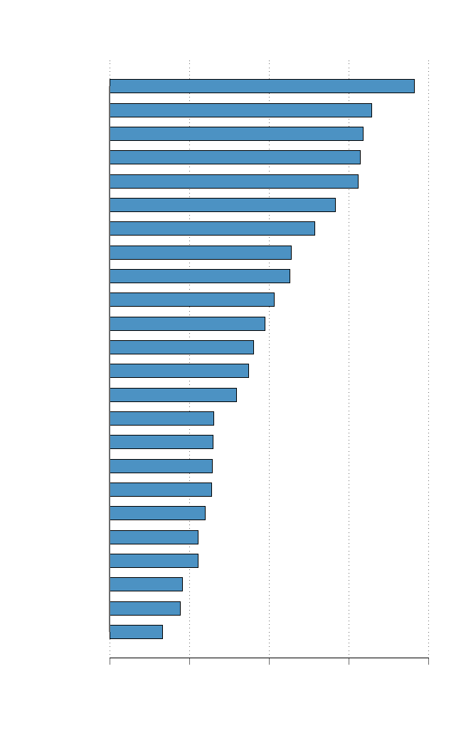
FIGURE A.3: CORPORATE TAX REVENUES IN OECD COUNTRIES, 2018

0 5 10 15 20

% of Total Revenue

United States

Italy

France

Germany

Greece

Finland

Austria

Denmark

Sweden

Iceland

United Kingdom

Turkey

Netherlands

Belgium

Czech Republic

Canada

Switzerland

Japan

Ireland

New Zealand

Korea

Luxembourg

Norway

Australia

Corporate Taxes as Share of Total Taxation

OECD Countries, 2018

Notes: This ﬁgure shows corporate tax revenues as a share of total taxation for OECD countries in 2018, using data from the OECD tax

database.

A.4 TCJA Tax Cut in the Context of Recent Literature

FIGURE A.4: TCJA TAX CHANGE VS. OTHER RECENT STUDIES

0 .05 .1 .15

Avg. Tax Change * Tax Base, as % of GDP

S-Seratto and Zidar 2016

(US State Corp Tax)

Giroud and Rauh 2019

(US State Corp Tax)

Fuest et al. 2019

(German Municipal Corp Tax)

This Paper

(US Federal Corp Tax)

Notes: This ﬁgure shows the average tax change studied in several recent papers, multiplied by the tax base and scaled by GDP. The

average tax change in Fuest et al. (2018) is 0.9 percentage points, and the LBT tax base is approximately 1.6% of GDP (see

OECD/UCLG 2019). The average tax change in Suárez Serrato and Zidar (2016) and Giroud and Rauh (2019) is 1.0 percentage point,

and the state corporate tax base is approximately 0.25% of GDP (Census 2019). The average tax change in this study is 9.0 percentage

points, and the 2016 federal corporate tax base is approximately 1.6% of GDP (OMB 2022).

A.5 Tax Rates for S-Corporations and Details of the QBI Deduction

TABLE A.2: PREDICTORS OF TAKE-UP OF THE QBI DEDUCTION FOR S-CORPS

(1) (2) (3)

2018 2019 Pooled

T I

-0.801

∗∗∗

-0.834

∗∗∗

-0.817

∗∗∗

(0.012) (0.011) (0.009)

SSTB (0/1) -0.110

∗∗∗

-0.068

∗∗∗

-0.090

∗∗∗

(0.025) (0.021) (0.020)

Proﬁts <=0 (0/1) -0.311

∗∗∗

-0.174

∗∗∗

-0.241

∗∗∗

(0.077) (0.059) (0.050)

Log Sales -0.014

∗∗∗

-0.008

∗∗

-0.011

∗∗∗

(0.004) (0.003) (0.003)

Outcome Mean 0.66 0.67 0.67

Year FE No No Yes

R2 0.59 0.67 0.63

N Firms 3,623 3,407 7,030

Notes: Table shows predictors of QBI takeup among

S-corporations.

A.6 Entity-Type Switching

TABLE A.3: ENTITY-TYPE SWITCHING

(1) (2)

S to C C to S

Log Lagged Sales × Post 0.000 0.004

(0.000) (0.002)

Firm Age × Post -0.000 -0.000

(0.000) (0.001)

Multinational (0/1) × Post 0.026

∗∗∗

-0.023

∗∗

(0.008) (0.010)

SSTB Industry × Post -0.001 0.016

(0.002) (0.026)

R2 0.00 0.02

N Firms 47,860 94,159

Notes: Table shows predictors of entity-type

switching after TCJA.

B Appendix to Section 3: Data Sources and Variable Deﬁnitions

B.1 Variable Deﬁnitions

Taxes Paid

Taxes paid are deﬁned for C-corporations as Form 1120: Schedule L, line 31. For S corps, taxes

paid are measured using the following methodology:

1. Match S-corp owners to their 1040s

2. Use 1040s to compute each owner’s average tax rate (ATR) and total taxes paid on pass-through income

(a) Calculate ATR for a tax unit: ATR = Taxes Paid / Taxable Income

(b) Record net ordinary business income: NET_OBI = Line 32 from 1040 (from schedule E)

1040)

(d) Save table unique by TIN-year

3. Compute total non-negative pass-through income from 1120s and 1065s by owner

(a) Append all K1s and from 1120s and 1065s with positive OBI (drop K1s with OBI<$0)

(b) Sum up OBI by TIN-year; call the sum OBI_SUM

4. Merge table 2 and 3 by TIN-year

5. Compute the OBI share of each pass-through business in the owner’s portfolio

(a) Append all K1s from 1120s with positive OBI

(b) Match m:1 by TIN with table 4; new table is unique by TIN-K1-year

(d) Allocate tax_paid in proportion to the shares: S_TAX = W*BIZ_TAX_PAID

(e) Sum up s_tax by ﬁrm-year, ﬁnal table is unique by EIN-year

Sales, Costs, and Proﬁts

Sales are deﬁned for C- and S-corporations as Form 1120: line 1c and Form 1120-S: line 1c,

respectively.

Costs of goods sold are deﬁned for C- and S- corporations as Form 1120: line 2 and Form 1120-S:

line 2, respectively.

Pre-tax gross proﬁts are deﬁned as sales minus costs of goods sold.

After-tax gross proﬁts are deﬁned as gross proﬁts minus taxes paid.

Earnings before interest, taxes, depreciation, and amoritization (EBITDA) is deﬁned as net

income plus net interest expense plus depreciation. Net income is deﬁned for C-corporations as

Form 1120: line 28. For S-corporations, net income is deﬁned as Form 1120-S: line 21 combined

with Form 1120-S Schedule K: lines 2 – 14. Depreciation is deﬁned for C- and S-corporations as

Form 1120: line 20 and Form 1120-S: line 14, respectively. Net interest expense is deﬁned for

C-corporations as the maximum of zero and Form 1120: line 18 minus line 5. For S-corporations,

net interest expense is deﬁned as Form 1120-S: line 12 plus Form 1120-S Schedule K: line 12b minus

line 4.

Shareholder Payouts

Dividends are deﬁned for C-corporations as Form 1120: Schedule M-2, line 5a plus line 5c. For

S-corporations, dividends are deﬁned as Form 1120-S: Schedule K, line 17c.

Share buybacks are deﬁned as the non-negative annual dollar change in the treasury stock;

treasury stock is deﬁned for C- corporations as Form 1120: Schedule L, line 27(d) and for

S-corporations as Form 1120-S: Schedule L, line 26(d).

Total payouts are deﬁned as dividends plus share buybacks.

Investment

Capital assets is deﬁned for C- and S- corporations as buildings and other depreciable assets less

accumulated depreciation, as measured on Form 1120: Schedule L, line 10b(d) and Form 1120-S:

Schedule L, line 10b(d), respectively.

Net investment is deﬁned as the annual dollar change in capital assets.

Short-life new investment is deﬁned for C- and S-corporations as the sum of Form 4562: lines

19a(c) to 19c(c).

Long-life new investment is deﬁned for C- and S-corporations as the sum of Form 4562 lines

19d(c) to 19i(c) plus the sum of lines 20a(c) to 20c(c) plus the sum of line 14, line 15, and line 16.

Total new investment is deﬁned as short-life new investment plus long-life new investment.

Employment and Earnings

Employment for C- and S-corporations is deﬁned as the total number of unique individuals with

a W-2 issued by the ﬁrm.

Worker earnings are measured for C- and S-corporation employees from Form W-2, box 5

(Medicare Wages).

Payroll is deﬁned as the sum of workers’ annual earnings.

Executive compensation is deﬁned for C-corporations as Form 1120: line 12 and for

S-corporations as Form 1120-S: line 7.

Top-5 compensation is deﬁned for C- and S-corporations as the combined annual W-2 earnings

of the top ﬁve highest paid workers at the ﬁrm.

Other Firm Characteristics

Age is deﬁned as tax year minus year of incorporation, where year of incorporation for

C-corporations and S-corporations is deﬁned as Form 1120: box C and Form 1120-S: box E,

respectively.

Multinational ﬁrms are deﬁned as those whose foreign sales share is greater than 1%, where

foreign sales are deﬁned as the sum of gross receipts from all Controlled Foreign Corporations

(that is, foreign subsidiaries) reported for each foreign subsidiary on Form 5471 Schedule C: line

1c.

Capital intensity is deﬁned at the industry level as total capital assets divided by total sales.

C- and S-corporations are classiﬁed as capital intensive if the mean of this ratio in the pre-period

(2013 to 2016) is greater than the sample median.

Industry is deﬁned for C-corporations as the ﬁrst three digits of Form 1120: Schedule K, line 2a

and for S-corporations as the ﬁrst three digits of Form 1120-S: Schedule B, line 2a.

B.2 Sample Distribution of Firms’ Statutory Marginal Income Tax Rates Before and

After TCJA

FIGURE B.1: SAMPLE DISTRIBUTION OF C-CORP STATUTORY MTR’S

Panel A: Marginal Tax Rates for C-Corporations

Percent

0 .1 .2 .3 .4

C-Corp Firm MTR

2016 2019

Panel B: Implied Marginal Tax Rates for S-Corporations

Percent

0 .1 .2 .3 .4

S-Corp Firm MTR

2016 2019

Notes: Table shows the sample distribution of statutory marginal income tax rates for C- and S-corps before and after TCJA.

B.3 Size Distribution of Capital-Intensive Industries

FIGURE B.2: SIZE DISTRIBUTIONS OF FIRMS, BY CAPITAL INTENSITY

Panel A: 2016 Sales

Density

$1mil $10mil $100mil $1bil $10bil $100bil

2016 Log Sales

Capital Intensive Not Capital Intensive

Panel B: 2016 Employment

Density

100 1K 10K 100K 1mil

2016 Log Employment

Capital Intensive Not Capital Intensive

Notes: Panels A and B show the distribution of 2016 log ﬁrm sales and employment, respectively, for capital-intensive and

non-capital-intensive ﬁrms.

C Appendix to Section 4: Empirical Results

C.1 Equity and Debt Issuance

TABLE C.1: EQUITY AND DEBT ISSUANCE

Equity Debt

(1) (2) (3) (4)

New Issuance (0/1) Log Issuance New Issuance (0/1) Log Debt

C × Post -0.003 0.027 0.005 -0.002

(0.006) (0.115) (0.008) (0.011)

2016 Outcome Mean 0.30 1.38 0.61 4.13

Firm FE Yes Yes Yes Yes

Industry-Size-Year FE Yes Yes Yes Yes

R2 81501 22633 81501 81299

N 11,647 4,950 11,647 11,639

Notes: Table shows result from estimating equation 2 to assess if TCJA caused increases in equity

or debt issuance of C-corps relative to S-corps. Columns 1 and 3 show the extensive margins, and

columns 2 and 4 show the intensive margins. We ﬁnd no signﬁciant difference.

C.2 Top 5 Earnings

TABLE C.2: TOP 5 EARNINGS

Outcome is top 5 earnings

Controls for:

Benchmark Sales Proﬁts Relative Sales

C × Post 0.040

∗∗∗

0.038

∗∗∗

0.038

∗∗∗

0.038

∗∗∗

(0.008) (0.008) (0.008) (0.008)

Firm FE Yes Yes Yes Yes

Industry-Size-Year FE Yes Yes Yes Yes

R2 1 1 1 1

N 81501 81501 81501 81259

N Firms 11,643 11,643 11,643 11,643

Notes: Unit of analysis is ﬁrm-year. Table reports results from estimating variations of equation 2, where the outcome is log

compensation of the top 5 highest paid workers at the ﬁrm. Column 1 shows the benchmark speciﬁcation, and columns 2-4 adds

time-varying controls for several measures of ﬁrm performance. Standard errors are clustered by ﬁrm.

C.3 Worker Heterogeneity

In Figure C.1 we explore whether the earnings effects of corporate statutory income tax cuts vary

across worker characteristics. Speciﬁcally, we test whether the annual earnings responses

estimated from equation 1 differ for men and women; for workers above and below the age of 40;

and for workers with above and below 5 years of work history with their employer in 2019. In

light of our previous evidence that earnings impacts vary across the within-ﬁrm earnings

distribution, we also condition on workers’ initial place in that distribution in 2016. For example,

in Panel A where the x-axis is 60, we estimate equation 1 separately for men and women who

were initially at the 60th percentile of the within-ﬁrm earnings distribution, and plot the resulting

2019

coefﬁcients and associated 95% conﬁdence intervals on the y-axis.

As can be seen from the

widely overlapping conﬁdence intervals in Figure ??, we do not ﬁnd compelling evidence that

treatment effects vary by gender, age, or employment tenure.

FIGURE C.1: WORKER HETEROGENEITY

Panel A: Gender Panel B: Age

2019

-.05

.05

20 40 60 80 100

Firm Wage Centile

Men Women

2019

-.05

.05

20 40 60 80 100

Firm Wage Centile

Age <40 Age>=40

Panel C: Tenure

2019

-.05

.05

20 40 60 80 100

Firm Wage Centile

<=5 Years Tenure >5 Years Tenure

Conditioning on workers’ initial place in the within-ﬁrm distribution requires that our sample is comprised of

“stayers”, that is, employees who worked at the same ﬁrm in 2016 and 2019.

C.4 Additional Investment Results

TABLE C.3: INVESTMENT SCALED BY 2016 BASELINE SALES

(1) (2) (3) (4) (5)

NetI

t−1

NewI

t−1

Short-Life Long-Life Structures

C × Post 0.008

∗∗∗

0.004 0.003

∗∗

-0.000 0.001

(0.003) (0.002) (0.001) (0.000) (0.001)

2016 Outcome Mean 0.01 0.06 0.04 0.01 0.01

Firm FE Yes Yes Yes Yes Yes

Industry-Size-Year FE Yes Yes Yes Yes Yes

R2 0.26 0.60 0.63 0.50 0.38

N 81,529 81,529 81,529 81,529 81,529

N Firms 11,647 11,647 11,647 11,647 11,647

Notes: Table shows results for new investment scaled by baseline sales. See Section 3 for variable

deﬁnitions.

C.5 Firm Heterogeneity

Event Studies for Capital Intensive vs. Non-Capital Intensive Industries

FIGURE C.2: SALES, COSTS, AND PRE-TAX PROFITS, BY CAPITAL INTENSITY

Panel A: Sales Panel B: Costs

-.05

.05

.15

2013 2014 2015 2016 2017 2018 2019

All Capital Intensive Not Capital Intensive

2016 Outcome Mean: 1.00

Sales / 2016 Sales

Difference Between C-Corps and S-Corps Over Time

-.05

.05

2013 2014 2015 2016 2017 2018 2019

All Capital Intensive Not Capital Intensive

2016 Outcome Mean: 0.53

Costs / 2016 Sales

Difference Between C-Corps and S-Corps Over Time

Panel C: Pre-Tax Proﬁts Panel D: EBITDA

-.05

.05

2013 2014 2015 2016 2017 2018 2019

All Capital Intensive Not Capital Intensive

2016 Outcome Mean: 0.47

Pre-Tax Profits / 2016 Sales

Difference Between C-Corps and S-Corps Over Time

-.1

2013 2014 2015 2016 2017 2018 2019

All Capital Intensive Not Capital Intensive

2016 Outcome Mean: 0.29

EBITDA / 2016 Sales

Difference Between C-Corps and S-Corps Over Time

Notes: Unit of analysis is ﬁrm-year. The panels plot the β

coefﬁcients from equation 1, estimated for all ﬁrms and separately for

capital-intensive and non-capital intensive industries. These coefﬁcients capture average differences in outcomes between C- and

S-corps over time after controlling for ﬁrm and industry-size-year ﬁxed effects. Standard errors are clustered by ﬁrm, and error bands

show 95% conﬁdence intervals. Sales are gross receipts. Costs are equal to cost of goods sold, including both material and labor costs.

Pre-tax proﬁts are sales minus costs. EBITDA is a harmonized measure of earnings before interest, taxes, depreciation, and

amoritization; see Section 3 and Appendix B for details.

FIGURE C.3: AFTER-TAX PROFITS AND SHAREHOLDER PAYOUTS, BY CAPITAL INTENSITY

Panel A: After-Tax Proﬁts

-.05

.05

.15

2013 2014 2015 2016 2017 2018 2019

All Capital Intensive Not Capital Intensive

2016 Outcome Mean: 0.41

After-Tax Profits / 2016 Sales

Difference Between C-Corps and S-Corps Over Time

Panel B: Shareholder Payouts (Extensive Margin)

-.04

-.02

.02

.04

.06

2013 2014 2015 2016 2017 2018 2019

All Capital Intensive Not Capital Intensive

2016 Outcome Mean: 0.54

Shareholder Payouts (0/1)

Difference Between C-Corps and S-Corps Over Time

Panel C: Shareholder Payouts (Intensive Margin)

-.2

2013 2014 2015 2016 2017 2018 2019

All Capital Intensive Not Capital Intensive

2016 Outcome Mean: 1.45

Log Shareholder Payouts

Difference Between C-Corps and S-Corps Over Time

Notes: Unit of analysis is ﬁrm-year. The panels plot the β

coefﬁcients from equation 1, estimated for all ﬁrms and separately for

capital-intensive and non-capital intensive industries. These coefﬁcients capture average differences in outcomes between C- and

S-corps over time after controlling for ﬁrm and industry-size-year ﬁxed effects. Standard errors are clustered by ﬁrm and error bands

show 95% conﬁdence intervals. In Panel A, after-tax proﬁts are deﬁned as pre-tax proﬁts minus tax, and are scaled by 2016 baseline

sales. In Panel B, the outcome is an indicator equal to 1 if shareholder payouts are positive (i.e., the extensive margin), where payouts

are deﬁned as the sum of cash and property distributions to shareholders. In Panel C, the outcome is log shareholder payouts (i.e., the

intensive margin). For additional information on data sources and variable deﬁnitions see Section 3 and Appendix B.

FIGURE C.4: LABOR MARKET OUTCOMES, BY CAPITAL INTENSITY

Panel A: Log Employment Panel B: Log Payroll

-.05

.05

2013 2014 2015 2016 2017 2018 2019

All Capital Intensive Not Capital Intensive

2016 Outcome Mean: 2,969

-.05

.05

2013 2014 2015 2016 2017 2018 2019

All Capital Intensive Not Capital Intensive

2016 Outcome Mean: 173

Panel C: Log Median Earnings Panel D: Log 99th Centile Earnings

-.03

-.02

-.01

.01

.02

.03

2013 2014 2015 2016 2017 2018 2019

All Capital Intensive Not Capital Intensive

2016 Outcome Mean: 46,278

-.05

.05

2013 2014 2015 2016 2017 2018 2019

All Capital Intensive Not Capital Intensive

2016 Outcome Mean: 371,861

Notes: Unit of analysis is ﬁrm-year. The panels plot the β

coefﬁcients from equation 1, estimated for all ﬁrms and separately for

capital-intensive and non-capital intensive industries. These coefﬁcients capture average differences in outcomes between C- and

S-corps over time after controlling for ﬁrm and industry-size-year ﬁxed effects. Standard errors are clustered by ﬁrm and error bands

show 95% conﬁdence intervals. The right panels are constructed such that the distance between the C-corp and S-corp lines in each

year is equal to the corresponding β

coefﬁcient in the left panel, and such that the observation-weighted average of the two lines is

equal to the unweighted sample average of the outcome in each year. For data sources and variable deﬁnitions see Section 3.

FIGURE C.5: EXECUTIVE PAY, BY CAPITAL INTENSITY

Panel A: Log Ofﬁcer Compensation

-.1

-.05

.05

2013 2014 2015 2016 2017 2018 2019

All Capital Intensive Not Capital Intensive

2016 Outcome Mean: 6,283,969

Panel B: Log Top 5 Earnings

-.05

.05

2013 2014 2015 2016 2017 2018 2019

All Capital Intensive Not Capital Intensive

2016 Outcome Mean: 1,186,758

Notes: Unit of analysis is ﬁrm-year. The panels plot the β

coefﬁcients from equation 1, estimated for all ﬁrms and separately for

capital-intensive and non-capital intensive industries. These coefﬁcients capture average differences in outcomes between C- and

S-corps over time after controlling for ﬁrm and industry-size-year ﬁxed effects. Standard errors are clustered by ﬁrm and error bands

show 95% conﬁdence intervals. For data sources and variable deﬁnitions see Section 3.

FIGURE C.6: INVESTMENT, BY CAPITAL INTENSITY

Panel A: Positive Net Investment (0/1)

-.05

.05

2013 2014 2015 2016 2017 2018 2019

All Capital Intensive Not Capital Intensive

2016 Outcome Mean: 0.52

Positive Net Investment (0/1)

Difference Between C-Corps and S-Corps Over Time

Panel B: Net Investment / Lagged Capital

-.05

.05

2013 2014 2015 2016 2017 2018 2019

All Capital Intensive Not Capital Intensive

2016 Outcome Mean: 0.06

Net Investment / Lagged Capital

Difference Between C-Corps and S-Corps Over Time

Panel C: New Investment / Lagged Capital

-.04

-.02

.02

.04

2013 2014 2015 2016 2017 2018 2019

All Capital Intensive Not Capital Intensive

2016 Outcome Mean: 0.25

New Investment / Lagged Capital

Difference Between C-Corps and S-Corps Over Time

Notes: Unit of analysis is ﬁrm-year. The ﬁgure plots the β

coefﬁcients estimated from equation 1. These coefﬁcients capture average

differences in outcomes between C- and S-corps over time after controlling for ﬁrm and industry-size-year ﬁxed effects. Standard

errors are clustered by ﬁrm and error bands show 95% conﬁdence intervals. Net investment is deﬁned as the change in book value of

depreciable capital assets minus accumulated book depreciation. New investment is measured as new capital expenditures; see

Section 3 for details. The outcome in Panel A is an indicator equal to 1 if net investment is positive. The outcomes in Panels B and C,

net and new investment, respectively, are scaled by lagged capital. For data sources and variable deﬁnitions see Section 3.

More Firm Heterogeneity

FIGURE C.7: FIRM HETEROGENEITY 1

Panel A Panel B

All

100-199 Emp

200-400 Emp

500-999 Emp

1000+ Emp

Low VA/Worker

High VA/Worker

Low Cash

High Cash

<10%

>10%

High Market Share

Low Market Share

Firm Size

Profitability

Liquidity

Unionization

Concentration

-.05 0 .05 .1 .15

Sales

All

100-199 Emp

200-400 Emp

500-999 Emp

1000+ Emp

Low VA/Worker

High VA/Worker

Low Cash

High Cash

<10%

>10%

High Market Share

Low Market Share

Firm Size

Profitability

Liquidity

Unionization

Concentration

-.04 -.02 0 .02 .04 .06

Costs

Panel C Panel D

All

100-199 Emp

200-400 Emp

500-999 Emp

1000+ Emp

Low VA/Worker

High VA/Worker

Low Cash

High Cash

<10%

>10%

High Market Share

Low Market Share

Firm Size

Profitability

Liquidity

Unionization

Concentration

-.05 0 .05 .1

Pre-Tax Profits

All

100-199 Emp

200-400 Emp

500-999 Emp

1000+ Emp

Low VA/Worker

High VA/Worker

Low Cash

High Cash

<10%

>10%

High Market Share

Low Market Share

Firm Size

Profitability

Liquidity

Unionization

Concentration

-.05 0 .05 .1

After-Tax Profits

Notes: The unit of analysis is a ﬁrm-year. The table shows the C × P ost coefﬁcients from equation 2. These coefﬁcients

estimate average differential changes in outcomes between C- and S-corps before and after TCJA controlling for ﬁrm

and industry-size-year ﬁxed effects (unless otherwise speciﬁed). Firm-size regressions include only industry-year ﬁxed

effects, and unionization regressions include only size-year ﬁxed effects. Standard errors are clustered by ﬁrm. Firms

are classiﬁed as high-cash if their mean ratio of liquid assets to assets in the pre-period is greater than the sample

median. Firms are classiﬁed as highly proﬁtable if their mean ratio of value-added per worker in the pre-period is

greater than the sample median. Firms are classiﬁed as highly-concentrated if their market share in industry sales in

the pre-period is greater than the sample median. Unionization rates are measured at the industry-level from the 2016

Current Population Survey.

FIGURE C.8: FIRM HETEROGENEITY 2

Panel A Panel B

All

100-199 Emp

200-400 Emp

500-999 Emp

1000+ Emp

Low VA/Worker

High VA/Worker

Low Cash

High Cash

<10%

>10%

High Market Share

Low Market Share

Firm Size

Profitability

Liquidity

Unionization

Concentration

-.1 0 .1 .2 .3 .4

Log Shareholder Payouts

All

100-199 Emp

200-400 Emp

500-999 Emp

1000+ Emp

Low VA/Worker

High VA/Worker

Low Cash

High Cash

<10%

>10%

High Market Share

Low Market Share

Firm Size

Profitability

Liquidity

Unionization

Concentration

-.02 0 .02 .04 .06 .08

Net Investment / Lagged K

Panel C Panel D

All

100-199 Emp

200-400 Emp

500-999 Emp

1000+ Emp

Low VA/Worker

High VA/Worker

Low Cash

High Cash

<10%

>10%

High Market Share

Low Market Share

Firm Size

Profitability

Liquidity

Unionization

Concentration

-.1 -.05 0 .05 .1

Log Employment

All

100-199 Emp

200-400 Emp

500-999 Emp

1000+ Emp

Low VA/Worker

High VA/Worker

Low Cash

High Cash

<10%

>10%

High Market Share

Low Market Share

Firm Size

Profitability

Liquidity

Unionization

Concentration

-.05 0 .05 .1

Log Payroll

FIGURE C.9: FIRM HETEROGENEITY 3

Panel A Panel B

All

100-199 Emp

200-400 Emp

500-999 Emp

1000+ Emp

Low VA/Worker

High VA/Worker

Low Cash

High Cash

<10%

>10%

High Market Share

Low Market Share

Firm Size

Profitability

Liquidity

Unionization

Concentration

-.03 -.02 -.01 0 .01 .02

Log Median Earnings

All

100-199 Emp

200-400 Emp

500-999 Emp

1000+ Emp

Low VA/Worker

High VA/Worker

Low Cash

High Cash

<10%

>10%

High Market Share

Low Market Share

Firm Size

Profitability

Liquidity

Unionization

Concentration

-.05 0 .05 .1 .15

Log 99th Centile Earnings

Panel C Panel D

All

100-199 Emp

200-400 Emp

500-999 Emp

1000+ Emp

Low VA/Worker

High VA/Worker

Low Cash

High Cash

<10%

>10%

High Market Share

Low Market Share

Firm Size

Profitability

Liquidity

Unionization

Concentration

-.05 0 .05 .1

Top 5 Earnings

All

100-199 Emp

200-400 Emp

500-999 Emp

1000+ Emp

Low VA/Worker

High VA/Worker

Low Cash

High Cash

<10%

>10%

High Market Share

Low Market Share

Firm Size

Profitability

Liquidity

Unionization

Concentration

-.05 0 .05 .1 .15

Executives' Compensation

C.6 Productivity

FIGURE C.10: PRODUCTIVITY

Panel A: Log Valued Added Per Worker

-.1

2013 2014 2015 2016 2017 2018 2019

All Capital Intensive Not Capital Intensive

2016 Outcome Mean: -3.74

Log Value Added Per Worker

Difference Between C-Corps and S-Corps Over Time

Panel B: Log Proﬁt Margin

-.1

-.05

.05

.15

2013 2014 2015 2016 2017 2018 2019

All Capital Intensive Not Capital Intensive

2016 Outcome Mean: -2.39

Log Profit Margin

Difference Between C-Corps and S-Corps Over Time

Notes: Unit of analysis is ﬁrm-year. The panels plot the β

coefﬁcients from equation 1, estimated for all ﬁrms and separately for

capital-intensive and non-capital intensive industries. These coefﬁcients capture average differences in outcomes between C- and

S-corps over time after controlling for ﬁrm and industry-size-year ﬁxed effects. Standard errors are clustered by ﬁrm, and error bands

show 95% conﬁdence intervals. Value added is deﬁned as EBITDA per worker. Proﬁt margin is deﬁned as the ratio of EBITDA to

sales. Standard errors are clustered by ﬁrm and error bands show 95% conﬁdence intervals.

C.7 2016-2019 Elasticities

TABLE C.4: ELASTICITIES ESTIMATED FROM TAX YEARS 2016-2019

(1) (2) (3) (4) (5) (6) (7)

Ln(1 − τ

MT R

) Pre-tax π Post-tax π I

t−1

p50

p95

Executives

ln(1 − τ

)× 2019 1.000

∗∗∗

0.508

∗∗∗

0.637

∗∗∗

0.927

∗∗∗

0.037 0.220

∗∗∗

0.701

∗∗∗

(0.000) (0.141) (0.150) (0.131) (0.071) (0.071) (0.214)

2016 Outcome Mean -0.31 0.47 0.41 0.06 46,278 157,639 6,283,969

Firm FE Yes Yes Yes Yes Yes Yes Yes

Industry-Size-Year FE Yes Yes Yes Yes Yes Yes Yes

N 81,529 81,529 81,529 81,529 81,529 81,529 72,400

N Firms 11,647 11,647 11,647 11,647 11,647 11,647 10,680

Notes: Table shows elasticities estimated using changes in outcomes between C- and S-corps from 2016-2019. These

estimates are unaffected by potential intertemporal shifting in tax years 2017 and 2018, and are similar to our

benchmark estimates.

C.8 Cost of Capital Elasticities

TABLE C.5: COST OF CAPITAL ELASTICITIES

(1) (2) (3) (4) (5) (6)

Pre-tax π Post-tax π I

t−1

p50

p95

exec

∆φ

× Post -0.669

∗∗∗

-0.920

∗∗∗

-0.910

∗∗∗

0.002 -0.312

∗∗∗

-1.128

∗∗∗

(0.224) (0.228) (0.145) (0.092) (0.094) (0.298)

2016 Outcome Mean 0.47 0.41 0.06 46,278 157,639 6,283,969

Firm FE Yes Yes Yes Yes Yes Yes

Industry-Size-Year FE Yes Yes Yes Yes Yes Yes

R2 81,529 81,529 81,529 81,529 81,529 72,400

N 11,647 11,647 11,647 11,647 11,647 10,680

Notes: Table shows cost-of-capital elasticities.

FIGURE C.11: THE EFFICIENCY-EQUITY TRADEOFF IN CONTEXT

Corp Income Tax

Personal Income Tax

Payroll Tax

Top 1% Share

of Tax Burden

More Efficient >>>

More Progressive >>

-.6 -.5 -.4 -.3 -.2 -.1 0

-1 * Elasticity of Taxable Income

Notes: The ﬁgure contextualized our results on the corporate income tax against the personal income and payroll taxes, the two other

largest sources of federal tax revenue in the United States. The elasticity of taxable income, shown on the X-axes, is a key parameter in

the literature for measuring tax distortions. The share of tax burden borne by the top of the income distribution is a measure of

progressivity.