
GE Healthcare
Biacore T200
Software Handbook

Biacore T200 Software Handbook 28-9768-78 Edition AA 1
Contents
1Introduction
1.1 System overview ............................................................................ 7
1.2 Support for use in regulated environments .............................. 8
1.3 Associated documentation .......................................................... 8
1.4 Biacore terminology ...................................................................... 8
2 Control Software – general features
2.1 Operational modes ...................................................................... 13
2.2 User interface ............................................................................... 14
2.2.1 Software help ............................................................................................. 15
2.3 Basic operation ............................................................................. 15
2.3.1 Selecting cycles and sensorgrams.................................................... 15
2.3.2 File menu...................................................................................................... 15
2.3.3 Edit menu ..................................................................................................... 17
2.3.4 View menu................................................................................................... 17
2.3.5 Run menu..................................................................................................... 19
2.3.6 Tools menu.................................................................................................. 19
2.3.7 Right-click menus ..................................................................................... 20
2.4 File storage .................................................................................... 21
2.4.1 Wizard templates and methods......................................................... 21
2.4.2 Result files.................................................................................................... 21
3Manual run
3.1 Preparing for a manual run ........................................................ 23
3.1.1 Instrument preparations ....................................................................... 23
3.2 Starting a manual run ................................................................. 24
3.3 Controlling a manual run ........................................................... 25
3.4 Ending a manual run ................................................................... 27
4 Application wizards
4.1 Wizard templates ......................................................................... 29
4.1.1 Creating and editing wizard templates .......................................... 29
4.1.2 Running wizards ....................................................................................... 30
4.2 Common wizard components .................................................... 30
4.2.1 Injection sequence ................................................................................... 30
4.2.2 Assay setup ................................................................................................. 32
4.2.3 Injection parameters............................................................................... 33
4.2.4 Sample and control sample tables ................................................... 34
4.2.5 System preparations............................................................................... 35
4.2.6 Rack positions............................................................................................ 37
4.2.7 Prepare Run protocol.............................................................................. 41
4.3 Wizard groups .............................................................................. 42
4.4 Immobilization pH scouting ....................................................... 42

2 Biacore T200 Software Handbook 28-9768-78 Edition AA
4.5 Immobilization ..............................................................................45
4.6 Regeneration scouting ................................................................50
4.7 Buffer scouting ..............................................................................54
4.8 Surface performance ...................................................................56
4.9 Binding analysis ............................................................................58
4.10 Concentration analysis ...............................................................61
4.11 Kinetics/Affinity ............................................................................65
4.12 Thermodynamics ..........................................................................70
4.13 Control experiments ....................................................................73
4.13.1 Mass transfer control.............................................................................. 73
4.13.2 Linked reactions control ........................................................................ 73
4.13.3 Evaluation of control experiments.................................................... 74
4.14 Immunogenicity ............................................................................76
5Methods
5.1 Opening methods .........................................................................77
5.2 Method structure ..........................................................................78
5.3 Method overview ..........................................................................79
5.4 General settings ............................................................................80
5.5 Assay steps ....................................................................................81
5.5.1 Base settings .............................................................................................. 82
5.5.2 Assay step preparations........................................................................ 84
5.5.3 Recurrence................................................................................................... 84
5.5.4 Number of replicates............................................................................... 85
5.6 Cycle types .....................................................................................86
5.6.1 Commands.................................................................................................. 87
5.6.2 Variables....................................................................................................... 93
5.6.3 Report points.............................................................................................. 95
5.7 Variable settings ...........................................................................97
5.8 Verification ....................................................................................98
5.9 Setup Run .......................................................................................98
5.9.1 Detection ...................................................................................................... 98
5.9.2 Variables....................................................................................................... 98
5.9.3 Cycle run list..............................................................................................100
5.9.4 System preparations.............................................................................100
5.9.5 Rack positions..........................................................................................101
5.9.6 Prepare Run Protocol............................................................................101
5.9.7 Starting the run .......................................................................................101
5.10 Requirements for assay-specific evaluation .........................101
5.10.1 Concentration analysis ........................................................................101
5.10.2 Kinetics/Affinity........................................................................................102
5.10.3 Thermodynamics....................................................................................102
5.10.4 Affinity in solution...................................................................................102
5.10.5 Immunogenicity ......................................................................................103
5.10.6 Other requirements ...............................................................................103

Biacore T200 Software Handbook 28-9768-78 Edition AA 3
6 Evaluation software – general features
6.1 User interface ............................................................................. 107
6.1.1 Organization .............................................................................................107
6.1.2 The Evaluation Explorer.......................................................................108
6.2 Basic operations .........................................................................108
6.2.1 Opening files .............................................................................................108
6.2.2 Printing evaluation results..................................................................109
6.3 Common display functions ....................................................... 109
6.3.1 Zooming the display..............................................................................109
6.3.2 Right-click menus ...................................................................................109
6.4 Predefined evaluation items .................................................... 112
6.4.1 Sensorgram...............................................................................................112
6.4.2 Plots..............................................................................................................112
6.5 Custom report points ................................................................113
6.5.1 Adding report points .............................................................................114
6.5.2 Editing and deleting report points...................................................115
6.6 Keywords .....................................................................................115
6.7 Solvent correction ......................................................................117
6.7.1 Background...............................................................................................117
6.7.2 When solvent correction should be used.....................................118
6.7.3 How solvent correction works ..........................................................119
6.7.4 Applying solvent correction................................................................119
6.8 Evaluation methods ...................................................................121
6.8.1 Creating evaluation methods............................................................121
6.8.2 Applying evaluation methods ...........................................................122
7 Data presentation tools
7.1 Sensorgram items ...................................................................... 123
7.1.1 Selecting sensorgrams for display..................................................124
7.1.2 Removing data ........................................................................................124
7.1.3 Sensorgram adjustment......................................................................125
7.1.4 Markers .......................................................................................................126
7.2 Plot items .....................................................................................127
7.2.1 Selector functions...................................................................................128
7.2.2 Table functions.........................................................................................129
7.2.3 Sorting the plot........................................................................................130
7.2.4 Fitting curves to points.........................................................................130
7.2.5 Adjusting plots for controls ................................................................132
7.2.6 Ranking .......................................................................................................134
7.3 Bar chart items ........................................................................... 135
7.3.1 Selector functions...................................................................................135
7.3.2 Display options ........................................................................................136
7.4 Report point table ...................................................................... 136
7.4.1 Displaying the report point table.....................................................136

4 Biacore T200 Software Handbook 28-9768-78 Edition AA
8 Concentration analysis
8.1 Requirements for concentration evaluation .........................141
8.1.1 Calibrated measurements..................................................................141
8.1.2 Calibration-free measurements.......................................................141
8.2 Evaluating calibrated concentration analyses .....................142
8.2.1 Calibration curves...................................................................................142
8.2.2 Calibration trends...................................................................................144
8.2.3 Control samples ......................................................................................146
8.2.4 Samples ......................................................................................................147
8.2.5 Custom models for calibration curves ..........................................148
8.2.6 Evaluating combined result sets.....................................................149
8.3 Evaluating calibration-free measurements ..........................150
8.3.1 Selecting samples...................................................................................150
8.3.2 Performing the evaluation..................................................................155
8.3.3 Interpreting the results.........................................................................156
8.3.4 Fitting model.............................................................................................157
9 Kinetics and affinity analysis
9.1 Requirements for kinetics and affinity evaluation ...............160
9.2 Evaluating kinetics and affinity in single mode ....................161
9.2.1 Basic procedure ......................................................................................161
9.2.2 Multiple ligand densities......................................................................169
9.3 Batch mode evaluation .............................................................170
9.4 Quality assessment for kinetics evaluation ..........................172
9.4.1 The Quality Control tab........................................................................172
9.4.2 Statistical parameters ..........................................................................175
9.4.3 Components of the fit ...........................................................................177
9.4.4 Check kinetic data..................................................................................177
9.5 Quality assessment for affinity evaluation ...........................179
9.6 Summarizing kinetics and affinity results .............................180
9.6.1 Creating kinetic summaries ...............................................................180
9.6.2 Basic summary presentation ............................................................180
9.6.3 On-off rate maps.....................................................................................183
9.7 Curve fitting principles ..............................................................184
9.7.1 Fitting procedure ....................................................................................184
9.7.2 Local and global parameters ............................................................185
9.8 Predefined models ......................................................................186
9.8.1 Kinetics – 1:1 binding............................................................................187
9.8.2 Kinetics – Bivalent Analyte .................................................................188
9.8.3 Kinetics – Heterogeneous Analyte ..................................................189
9.8.4 Kinetics – Heterogeneous Ligand....................................................191
9.8.5 Kinetics – Two State Reaction...........................................................193
9.8.6 Affinity – Steady State 1:1...................................................................195
9.9 Creating and editing models ....................................................195
9.9.1 Interaction models for kinetics .........................................................196
9.9.2 Equation models for kinetics .............................................................200
9.9.3 Models for steady state affinity ........................................................202

Biacore T200 Software Handbook 28-9768-78 Edition AA 5
10 Thermodynamic analysis
10.1 Background .................................................................................203
10.1.1 Equilibrium thermodynamics ............................................................203
10.1.2 Transition state thermodynamics ...................................................204
10.2 Performing thermodynamic analysis ..................................... 205
11 Affinity in solution
11.1 Conventions and background ..................................................209
11.1.1 Experimental setup................................................................................209
11.1.2 Evaluation principles.............................................................................209
11.2 Requirements for affinity in solution ......................................210
11.3 Evaluation of affinity in solution .............................................211
12 Immunogenicity
Appendix A Data import and export
A.1 Exporting data ............................................................................217
A.1.1 Export functions ......................................................................................217
A.2 Importing data ............................................................................ 218
A.2.1 Control Software.....................................................................................218
A.2.2 Evaluation Software..............................................................................221
Appendix B Method examples and recommendations
B.1 Affinity in solution ...................................................................... 223
B.2 Calibration-free concentration analysis ................................224
B.2.1 Assay steps and general settings....................................................224
B.2.2 Cycle types.................................................................................................224
B.2.3 Variable settings......................................................................................225
B.2.4 Setup Run...................................................................................................226
B.3 CAP single-cycle kinetics ..........................................................227
B.3.1 Assay steps................................................................................................227
B.3.2 Sample analysis cycle for Sensor Chip CAP................................228
B.4 GST kinetics .................................................................................230
B.5 Inject and Recover .....................................................................232
B.6 Kinetics heterogeneous analyte .............................................. 234
B.7 L1 liposome capture .................................................................. 234
B.8 LMW kinetics and LMW Screen ................................................235
B.9 LMW single-cycle kinetics ........................................................237
B.10 Single-cycle kinetics .................................................................. 237
Index.............................................................................................. 239

6 Biacore T200 Software Handbook 28-9768-78 Edition AA

Biacore T200 Software Handbook 28-9768-78 Edition AA 7
Introduction 1
1 Introduction
Biacore™ T200 is a high performance system for analysis of biomolecular
interactions, based on GE Healthcare’s surface plasmon resonance (SPR)
technology. The Control Software supplied with the system offers easy-to-use
wizards for assay development and common applications together with flexible
facilities for designing custom analysis methods using a graphical interface
called Method Builder. Results are evaluated in separate Evaluation Software
designed for efficient and flexible evaluation, with dedicated functions for
common applications.
This Handbook describes in detail how to use the Control and Evaluation
Software.
1.1 System overview
Instrumentation in the Biacore T200 system is described in full in the
Biacore T200 Instrument Handbook. Important features relevant to software
operation include:
• Biacore T200 supports simultaneous analysis in up to four flow cells
connected in series. The flow cells are arranged in pairs (Fc1-2 and Fc3-4)
with minimum dead volume between the flow cells in a pair to provide
accurate reference subtraction.
• The sample compartment accommodates one microplate (96- or 384-well,
regular or deep-well capacity) and one reagent rack for reagent vials. A
combined sample and reagent rack can be used in place of the separate
microplate and reagent rack.
• Material that binds to the sensor surface during sample injection can be
recovered in a small volume of liquid for further analysis by e.g. mass
spectrometry.
• The temperature in the sample compartment is controlled separately from
the analysis temperature, allowing samples to be kept at one temperature
while analysis is performed at another. Samples equilibrate to the analysis
temperature during injection into the flow cell. The analysis temperature
can be varied during a run, and the sample compartment temperature
can be set to follow the analysis temperature if desired.
• The system includes a buffer selector valve, allowing analysis to be
performed in up to four different buffers in the same unattended run.

1 Introduction
1.2 Support for use in regulated environments
8 Biacore T200 Software Handbook 28-9768-78 Edition AA
1.2 Support for use in regulated environments
Support for use in regulated (GxP
1
) environments is provided in an optional
package that adds appropriate functionality to the Biacore T200 software.
Functions for GxP support are described in a separate Biacore T200 GxP
Handbook. Descriptions of software in the current Handbook apply to
installations both with and without the GxP package unless otherwise stated.
1.3 Associated documentation
This Handbook describes Biacore T200 Control Software and Evaluation
Software, version 1.0. Any functionality that is added in optional add-on
modules is described in separate documentation.
Biacore T200 Instrument Handbook describes the instrumentation in the
Biacore T200 system, with instructions for operation, maintenance and
troubleshooting.
Biacore T200 GxP Handbook describes functionality added with the optional
GxP package, together with some recommendations for using the system in a
regulated environment.
Biacore T200 Immunogenicity Handbook describes the use of specialized
functions in the software for immunogenicity studies.
Other general handbooks and documentation describing the technology are
available from GE Healthcare. Information may also be found on the Internet at
www.gelifesciences.com/biacore.
1.4 Biacore terminology
Biacore monitors the interaction between two molecules, of which one is
attached to the sensor surface and the other is free in solution. The following
terms are used in the context of work with Biacore systems (see Figure 1-1):
• The partner attached to the surface is called the ligand. Attachment may
be covalent or through high affinity binding to another molecule which is
in turn covalently attached to the surface. In the latter case the molecule
attached to the surface is referred to as the capturing molecule.
Note: The term “ligand” is applied here in analogy with terminology used in
affinity chromatography contexts, and does not imply that the
surface-attached molecule is a ligand for a cellular receptor.
•The analyte is the interacting partner in solution for which the
concentration is to be measured. In direct binding assays, the analyte
1
GxP is used as a generic abbreviation for GLP (Good Laboratory Practice), GMP (Good
Manufacturing Practice) and GCP (Good Clinical Practice).

Biacore T200 Software Handbook 28-9768-78 Edition AA 9
Introduction 1
binds directly to the ligand. In inhibition assays, the concentration of
analyte is measured indirectly through binding of an additional molecule.
Figure 1-1. Ligand, analyte and capturing molecule in relation to the sensor surface.
• Regeneration is the process of removing bound analyte from the surface
after an analysis cycle without damaging the ligand, in preparation for a
new cycle.
• Response is measured in resonance units (RU). The response is directly
proportional to the concentration of biomolecules on the surface.
•A sensorgram is a plot of response against time (see Figure 1-2), showing
the progress of the interaction. This curve is displayed directly on the
computer screen during the course of an analysis. Sensorgrams may be
analyzed to provide information on the rates of the interaction.
• In many assay situations, sample passes over two or more flow cells in
series, where one flow cell (usually the first) serves as a reference while
ligand is attached in the other flow cell(s). Surfaces with ligand are referred
to as active: blank surfaces used for reference purposes are reference.
• A particular sensorgram is referred to as a curve in several contexts in the
software. This terminology is used to distinguish between different classes
of sensorgram that recur within a run: for example, measurements on one
active and one reference surface can generate separate curves for each
of the two flow cells and a third reference-subtracted curve (active minus
reference)
•A report point records the response on a sensorgram at a specific time
averaged over a short time window, as well as the slope of the sensorgram
over the window. The response may be absolute (above a fixed zero level
determined by the detector) or relative to the response at another
specified report point.

1 Introduction
1.4 Biacore terminology
10 Biacore T200 Software Handbook 28-9768-78 Edition AA
Figure 1-2. Schematic illustration of a sensorgram. The bars below the sensorgram
curve indicate the solutions that pass over the sensor surface.

Biacore T200 Software Handbook 28-9768-78 Edition AA 11
Control Software

12 Biacore T200 Software Handbook 28-9768-78 Edition AA

Biacore T200 Software Handbook 28-9768-78 Edition AA 13
Control Software – general features 2
2 Control Software – general features
2.1 Operational modes
Biacore T200 Control Software offers three modes of operation:
• Manual run provides interactive control of the instrument operation,
executing commands singly as they are issued. This mode is most useful
for ad hoc experiments involving one or a few injections, such as testing
the response obtained from injection of a single sample.
• Application wizards provide guidance in setting up experiments for assay
development and execution. Separate wizards are offered for different
purposes such as ligand immobilization, concentration determination or
measurement of kinetic constants. Each wizard consists of an ordered
series of dialog boxes, ensuring that the essential features of the
application setup are correctly defined.
• Methods provide greater flexibility (and conversely less guidance) in setting
up applications, allowing customized applications that are not covered by
wizards. Methods are defined in a graphical interface called Method
Builder, which is designed to provide full flexibility in method definition
while retaining a simple interface for running assays based on established
methods. Application wizard templates may be opened in Method Builder
to provide a starting point for further refinement of application setup.
Predefined methods are also provided as help in defining methods for
selected purposes (see Appendix B).
Each of these modes of operation is described in more detail in the following
chapters.

2 Control Software – general features
2.2 User interface
14 Biacore T200 Software Handbook 28-9768-78 Edition AA
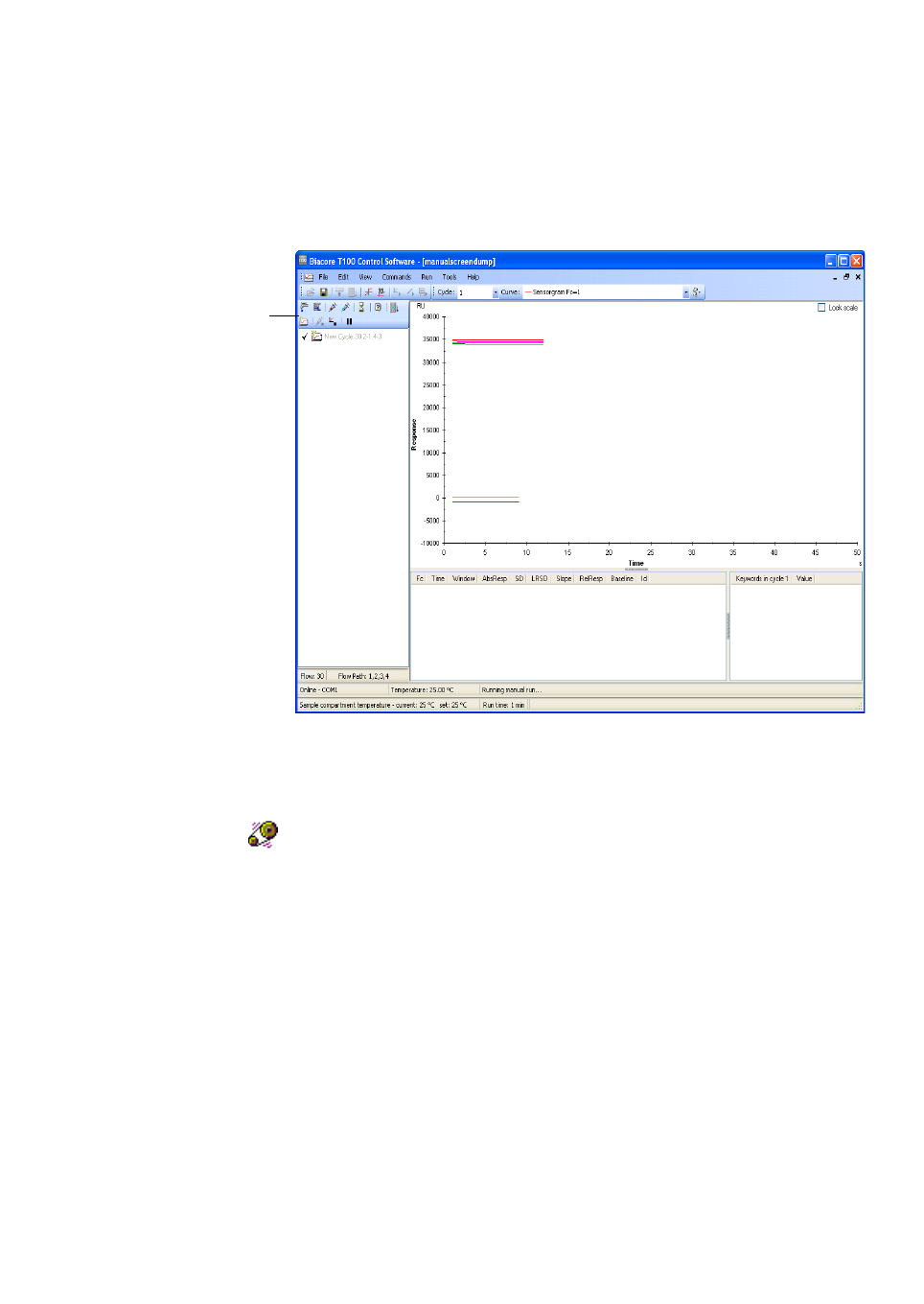
2.2 User interface
The main screen in the control software is divided into the following areas
•The menu and toolbar provide access to control commands.
•The event log records settings at the start of the run and instrument
control events during the run. The event log is displayed in a separate
window, opened by clicking on the Event Log button at the right of the
toolbar.
•The sensorgram window displays the sensorgrams for the current run or
the currently open file.
•The report point table lists report points for the currently displayed cycle.
Report points record the response at a set time and are defined
automatically: custom report points can also be added in methods, or
after the run in either the Control Software or the Evaluation Software.
•The keyword table lists keywords for the currently displayed cycle.
Keywords are defined automatically in wizard runs, or in the method for
method runs.
•The status bar displays the instrument status, including the temperature of
the detector and the sample compartment. The content of the status bar
varies between different situations: for wizard- and method-based runs,
the elapsed run time and the estimated total run time are included.
Menu and toolbar
Event log
Sensorgram window
Report point table
Keyword table
Status bar

Biacore T200 Software Handbook 28-9768-78 Edition AA 15
Control Software – general features 2
2.2.1 Software help
Software help is available at any time from the Help menu. Context-specific help
for dialog boxes is provided through Help buttons in the boxes.
2.3 Basic operation
2.3.1 Selecting cycles and sensorgrams
During a run, the current cycle is displayed by default. You can choose which
cycle to display in the Cycle selector, but the display will revert to the current
cycle when a new cycle is started. For a completed run, choose which cycle to
display with the Cycle selector in the toolbar:
The Curve selector determines which curve in the cycle is current in the display.
Options in the View menu (Section 2.3.4) control which curves are displayed in
the sensorgram window.
2.3.2 File menu
The Open/New options for wizard templates and methods create new wizard
templates and methods, and open existing templates and methods for editing
or for starting a run.
Open opens result files. Most result files just display the sensorgrams and tables.
Files from immobilization and regeneration scouting wizards also display a
summary window showing the results of the run (see Sections 4.5 and 4.6).
Save and Save As save the results as a Biacore results file (extension .blr).
Export exports the current results to a file in Microsoft Excel or XML format, or
exports the contents of the report point table to a tab-separated file. See
Appendix A for details of the export format.

2 Control Software – general features
2.3 Basic operation
16 Biacore T200 Software Handbook 28-9768-78 Edition AA
Print prints a hard-copy of the results. Select the printer to use and check the
items you wish to print.
Sensorgrams may be printed as follows:
Note: In order to maintain report layout, the print orientation is fixed regardless
of the printer settings in Windows.
Properties shows detailed properties of the currently opened run, including the
properties of the sensor chip used in the run.
When you close the software with Exit while the instrument is still switched on,
you may choose to shut down the instrument for a shorter or longer period if
required. See the Biacore T200 Instrument Handbook or the on-line help for
more details.
None No sensorgrams will be printed.
Current cycle The current cycle will be printed with the View:Show… setting
and scale as shown on the screen.
Range and
All cycles
Multiple cycles will be printed. For Range, enter a range or
cycle numbers separated by commas (e.g. 4-16,19,22).
All curves will be included in each cycle regardless of the
View:Show… setting. Sensorgrams will be printed at full scale
unless the Lock Scale box is checked in the sensorgram
window, in which case the current scaling will be applied to
all cycles (with this setting, some sensorgrams may appear to
be empty).

Biacore T200 Software Handbook 28-9768-78 Edition AA 17
Control Software – general features 2
2.3.3 Edit menu
Options in the Edit menu allow you to add, edit and delete report points. Report
points are created automatically and are used in various evaluation contexts.
You should in general avoid editing or deleting report points that are created
automatically.
Editing operations for report points in the Control Software may be applied to
single report point instances or to all instances of the report point in the current
cycle. Note that editing operations are not applied to multiple cycles.
Report points created in the Control Software cannot be edited in the Evaluation
Software. The Evaluation Software offers functions for creating and editing
custom report points that can be applied to all cycles in the run in a single
operation. This is usually preferable to adding report points in the Control
Software.
2.3.4 View menu
Chip Properties opens a dialog box that displays the properties of the currently
docked sensor chip. The Ligand column is empty for flow cells that have not
been used, and shows [Blank] for flow cells that have been prepared as a blank
reference surface by activation and deactivation. The text [Incomplete results]
indicates that the immobilization run was interrupted (by for instance user
intervention or power failure) before it could be completed.

2 Control Software – general features
2.3 Basic operation
18 Biacore T200 Software Handbook 28-9768-78 Edition AA
Properties for the sensor chip used in a currently open run may be found under
File:Properties (Section 2.3.2).
Title sets a title in the sensorgram window. The default title is the assay step
name.
Scale sets the scale of the sensorgram window:
If you set Auto scale, the scale will be adjusted if necessary to accommodate
the full data range of the currently displayed cycle. During a run, the scale is
adjusted at intervals as more data is collected. Check the Lock scale box in the
top right corner of the sensorgram window to lock the scale to the current
settings.
Adjust Scale sets the scale to the full data range. This will not affect the Auto
scale setting in the Scale dialog. Adjust Scale overrides but does not turn off the
Lock scale setting.
To scale the sensorgram display interactively, drag with the cursor over the area
to be scaled. Double-clicking in the display or choosing View:Unzoom restores
the previous zoom setting.
Reference line toggles display of a movable vertical line in the sensorgram
window, together with a separate small window that shows the response and
time coordinates at the reference line for the current curve. Use the Curve
selector in the toolbar (see Section 2.3.1) to set the current curve. Drag the
reference line to move it. When the reference line is displayed, choosing
Baseline sets a baseline at the current reference line position, and the
coordinates window shows the response relative to that baseline.

Biacore T200 Software Handbook 28-9768-78 Edition AA 19
Control Software – general features 2
The options Show Only Current Curve, Show Curves of Same Type and Show
All Curves control which curves are displayed in the sensorgram window. Curve
types distinguish between unsubtracted and reference-subtracted curves.
Choose the Event Log option or click on the Event Log button at the right of the
toolbar to display the event log window.
Choose the Wizard Template or Method options to display the wizard or
method definition for the run. You can edit the definition and save it as a new
wizard template or method. You cannot however change the original definition
that is saved together with the result file.
Notebook opens a notebook window where details of the run may be recorded.
The notebook is only available during a run or for a completed result file. The run
notebook is saved with the result file and can be viewed in the Evaluation
Software.
For some wizard runs and for test tools, the Wizard Results option opens a
window showing the results of the run. All other runs are evaluated in the
Evaluation Software.
Sensorgram Markers controls display of report point and event markers and
labels in the sensorgram window.
2.3.5 Run menu
The options in the Run menu are used to start the different types of runs (see
Chapters 3–5.
2.3.6 Tools menu
Options in the Tools menu control instrument operations outside the context of
runs.
Prime flushes the flow system with fresh buffer. There is an option to include
Prime at the beginning of each wizard- or method-based run. Use the menu
option when you want to flush the system at other times (e.g. before a manual
run).
Shutdown starts the procedure for shutting down the instrument for long
periods of time (more than 7 days). The procedure displays necessary
instructions on the screen. Details of the shutdown procedure are given in the
Biacore T200 Instrument Handbook.
Standby puts the instrument in standby mode, which maintains a low buffer or
water flow through the flow system for up to 7 days. Leaving the instrument in
standby mode when not in use is generally recommended. The instrument is

2 Control Software – general features
2.3 Basic operation
20 Biacore T200 Software Handbook 28-9768-78 Edition AA
automatically put in standby mode at the end of a run. Use the menu option if
standby has been stopped and you want to restart it.
Stop Standby stops standby mode.
Eject Rack ejects the rack tray from the sample compartment. The rack may be
ejected during setup for wizard- and method-based runs, and at any time
during a manual run. Use the menu option or the toolbar button when you want
to eject the rack at any other time.
Rack Illumination switches the illumination in the sample compartment on or
off. The illumination helps you to see in the sample compartment but does not
otherwise affect instrument function.
Insert Chip and Eject Chip are used for docking and undocking the sensor chip
respectively. More details are given in Chapter 4 of the Biacore T200 Instrument
Handbook.
Set Temperature sets the sample compartment and analysis temperature.
More details are given in Chapter 4 of the Biacore T200 Instrument Handbook.
Preferences controls aspects of file storage and data import (see Section 2.4),
and the time to automatic retraction of the rack tray.
More Tools provides access to maintenance, test and service tools. Details are
given in Appendix B of the Biacore T200 Instrument Handbook.
2.3.7 Right-click menus
Right-clicking with the mouse in many windows opens context menus specific
for the window.
Sensorgram window
Scale opens the same dialog as the View:Scale option (Section 2.3.4).
Copy Graph copies the sensorgram window exactly as displayed to the
Windows clipboard. Use this option to insert a copy of the sensorgram window
into other programs such as presentation software.
Export Curves exports data for the currently displayed curves to a text file.
Entire curves are exported regardless of the scale of the display. The exported
data includes report points and event marker times if these are displayed in the
sensorgram window. See Appendix A for more details of the export format.
CAUTION
The rack tray automatically moves into the instrument a preset time after it
has been ejected. The time to auto-close is set in Tools:Preferences.
A timer in the dialog indicates when the rack tray will be automatically
moved into the instrument.

Biacore T200 Software Handbook 28-9768-78 Edition AA 21
Control Software – general features 2
Gridlines controls display of gridlines in the sensorgram window.
Report point table
The right-click menu options for the report point table correspond to the
Edit:Report Points menu options.
Notebook
Right-click menu options in the notebook represent standard Windows editing
functions.
2.4 File storage
2.4.1 Wizard templates and methods
Wizard templates are saved in files with a file name extension .bw**, where **
represents an abbreviation that identifies the wizard (e.g. a wizard template for
concentration analysis has the extension .bwConc).
Methods are saved in files with the file name extension .Method.
Note: The extension will not be displayed if the setting Hide file extensions for
known file types is selected in the Windows Explorer folder options.
Turning this setting off can help you to identify file types in dialog boxes.
Templates and methods may be saved in any location when the optional
Biacore T200 GxP Package is not installed. A folder structure under the default
location as specified on the Folders tab in Tools:Preferences is however
recommended, since files in this location are handled preferentially in the
Open/New dialog boxes for wizards and templates (see Section 4.1.1).
2.4.2 Result files
Results are saved in files with the file name extension .blr. Result files from
wizard- or method-based runs contain a copy of the wizard template or method
as well as the results of the run.

2 Control Software – general features
2.4 File storage
22 Biacore T200 Software Handbook 28-9768-78 Edition AA

Biacore T200 Software Handbook 28-9768-78 Edition AA 23
Manual run 3
3 Manual run
Manual run allows you to control a run interactively. All settings except
temperature and choice of microplate and/or reagent rack can be changed
during the run. Commands are placed in a queue if the instrument is busy when
a command is issued: queued commands that have not yet been started can be
edited or deleted from the queue.
The results of a manual run are saved in a normal result file, and can be
evaluated in the Evaluation Software. There are however no predefined
keywords associated with the run, and the results cannot be evaluated with the
Evaluation Software tools for concentration, kinetics/affinity, thermodynamics
or immunogenicity.
3.1 Preparing for a manual run
3.1.1 Instrument preparations
The integrated instrument preparation steps that are included with wizard- and
method-based runs are not supported for manual run. The instrument should
therefore be prepared using options from the Tools menu.
1 Dock the chip that you want to use, and immobilize ligand on the surface
(see Section 4.5) if this has not already been done.
2Choose Tools:Prime to flush the flow system with fresh buffer.
3Choose Normalize from the Maintenance Tools section of Tools:More
Tools if the detector has not been normalized since the chip was docked. (In
many cases, the detector will have been normalized in connection with
ligand immobilization. However, you may need to perform the operation
again if the chip has been undocked and re-docked after immobilization.)
4Choose Tools:Set Temperature and set the analysis and sample
compartment temperatures. Wait until the analysis temperature is stable
(as shown in the status bar) before starting the run.
5 Prepare your samples and reagents in the microplate and/or reagent rack.
Note the rack positions and volumes of samples that you prepare: there is
no software support in manual run for identifying samples or monitoring
the volume of liquid in the autosampler positions. You insert the samples as
part of the starting procedure for the run. You can also add samples during
the run.

3Manual run
3.2 Starting a manual run
24 Biacore T200 Software Handbook 28-9768-78 Edition AA
3.2 Starting a manual run
Choose Run:Manual Run to start a manual run.
Choose the initial settings for flow rate, flow path and reference subtraction. You
can change the flow rate at any time during the run. You can change the flow
path at any time: during a cycle, the available options are restricted by the
choice made when the cycle is started.
Choose the rack and microplate settings. These will apply throughout the run
and cannot be changed.
Click Eject Rack to eject the rack tray so that you can load your samples.
Click Start to start the run. You will be asked to specify a result file name before
the run actually starts.
Biacore T200 Software Handbook 28-9768-78 Edition AA 25
Manual run 3
3.3 Controlling a manual run
Control the manual run from the command buttons in the main window or the
options in the Command menu:
Commands are executed immediately if the instrument is idle. With a few
exceptions (noted in the detailed descriptions below), commands issued when
the instrument is busy are placed at the end of a queue. The queue is listed in
the left-hand panel, with commands that have been executed in gray text and
those that are pending in black text. The command currently being executed is
marked with a “working” icon.
Right-click on a pending command for a menu with options for:
• editing the command
• inserting a new command before the selected command (you choose the
command to insert from a dialog box)
• deleting the command
You can also use the right-click menu to copy selected command or commands
and paste them elsewhere in the queue. The Copy function works with both
completed and pending commands.
Command
buttons

3Manual run
3.3 Controlling a manual run
26 Biacore T200 Software Handbook 28-9768-78 Edition AA
Flow rate
Sets the flow rate to a new value.
Flow path
Changes the flow path. During a cycle, you can only select a flow path within a
range allowed by the setting chosen when the cycle was started (for example, if
the current setting is Flow path 1-2, you cannot extend it to Flow path 1-2-3-4).
Sample injection
Injects sample. Choose the position from which the sample will be taken and
specify a contact time. Positions that can be chosen are determined by the rack
settings in the manual run start-up dialog. Make sure that the chosen position
contains enough sample for the injection. The required volume for the specified
contact time is indicated in the dialog box.
Regeneration injection
Injects regeneration solution. Choose the position from which the solution will be
taken and specify a contact time. Positions that can be chosen are determined
by the rack settings in the manual run start-up dialog. Make sure that the
chosen position contains enough solution for the injection. The required volume
for the specified contact time is indicated in the dialog box.
Check High viscosity solution if your regeneration solution has a relative
viscosity higher than about 3 (corresponding to about 35% glycerol or 40%
ethylene glycol at 20°C). This will adjust the injection procedure to ensure correct
handling of viscous solutions, and will limit the maximum contact time that can
be specified.
Wait
Inserts a Wait command in the queue, causing the instrument operation to
pause for the specified time period. Buffer continues to flow over the sensor
surface during the Wait period and data collection continues.
Eject Rack Tray
Ejects the rack tray so that you can load more samples. Do not change the type
of microplate or reagent rack on the tray.
This command is inserted immediately after the command currently under
execution, rather than at the end of the queue, so that the rack tray will be
ejected as soon as the current command is completed. If you want to place the
command later in the queue, use the right-click menu in the queue panel to
insert the command at the appropriate place.

Biacore T200 Software Handbook 28-9768-78 Edition AA 27
Manual run 3
New Cycle
Starts a new cycle. You can choose a new flow path and reference subtraction
setting for the new cycle, independently of the setting in the current cycle.
Stop <command>
Stops the command currently being executed. The icon changes to show the
command that will be stopped, or is gray if the current command cannot be
stopped (e.g. it is not possible to stop an Eject Rack Tray command).
Stop Run
Finishes the run.
Pause Run
Pauses the run until a Resume Run command is issued. Buffer continues to flow
over the sensor surface while the run is paused. Data collection continues
during the pause.
Resume Run
Resumes a run that is paused.
Add report point
Adds a report point to the sensorgram.
Help
Displays help for the manual run.
3.4 Ending a manual run
To end a manual run:
1Issue a Stop Run command. The command will normally be placed at the
end of the queue. If you want to stop the run before the queue is completed,
use the right-click menu in the queue panel to delete commands from the
queue or to insert the Stop Run command in the appropriate position.
2Choose Tools:Eject Rack to eject the rack tray and remove your samples
and reagents.
3Choose Tools:Eject Chip to undock the chip if desired.

3Manual run
3.4 Ending a manual run
28 Biacore T200 Software Handbook 28-9768-78 Edition AA

Biacore T200 Software Handbook 28-9768-78 Edition AA 29
Application wizards 4
4 Application wizards
Application wizards guide you through the procedure of setting up common
applications, with recommendations and settings based on GE Healthcare’s
expertise in the field of SPR-based interaction studies. Wizards are an ideal
starting point for inexperienced or infrequent users, since they offer a structured
sequence of settings that covers all essential aspects of the assay in question.
Wizard settings can be saved in templates for later use. Advanced users can
open wizard templates in Method Builder for more flexible assay design (see
Chapter 5).
4.1 Wizard templates
An application wizard consists of a series of dialog boxes that takes you through
the steps in setting up the application. Settings in the dialog boxes may be saved
in wizard templates, so that opening a template will present the saved settings
in each dialog box.
Normally, a wizard template is saved when all steps have been defined, so that
the template represents a complete assay definition including sample details if
desired. If a wizard sequence is closed before reaching the last step, however,
you are given an opportunity to save the template, which will then contain
settings as far as they have been defined.
4.1.1 Creating and editing wizard templates
To create a new wizard template or edit an existing template, choose
File:Open/New Wizard Template and select the type of wizard in the dialog box.
Click New to create a new template, or navigate to the folder where your
template is stored, select the template and click Open to edit an existing
template.
The top-level folder for wizard templates is defined under Tools: Preferences
(see Section 2.4). You can navigate between subfolders under the top level in the
dialog box, but you cannot access templates outside the top-level folder directly
from within the dialog box. Click Browse to navigate freely in the computer file
structure and open wizard templates stored in other locations.
Note: The Open/New Wizard Template dialog box only lists templates of the
selected type, but the Browse dialog may list all types. Template types are
identified by the file extension, which may or may not be displayed
according to your Windows Explorer settings (see Section 2.4.1).

4 Application wizards
4.2 Common wizard components
30 Biacore T200 Software Handbook 28-9768-78 Edition AA
4.1.2 Running wizards
When you start a run based on a wizard template, the template settings are
displayed as you step through the wizard. You can change settings for the
particular run if desired: the changes are not saved in the wizard template
unless you explicitly request this with the Save wizard template option. Setting
used for the run are stored in the result file and can be examined and saved as
a new wizard template from the completed run.
4.2 Common wizard components
Several dialogs are common to a number of wizards, with equivalent functions
and only minor differences. These dialogs are described in the current section.
Any wizard-specific variations in these common components are described in
the sections on the respective wizards below.
4.2.1 Injection sequence
This dialog determines the sequence of injections in the wizard analysis cycle.
Some injections are not supported in certain wizards (e.g. the kinetics wizard
does not support enhancement injections).
Detection settings
Select the flow path for the analysis. The setting will apply throughout the whole
wizard run. The available flow paths vary between the different wizards
according to wizard purpose.

Biacore T200 Software Handbook 28-9768-78 Edition AA 31
Application wizards 4
The detection is automatically set to the same settings as the flow path, so that
sensorgrams are recorded only from the flow cells used.
When reference subtraction is used together with ligand capture (Section 4.2.1),
the captured ligand passes over the active surface but not the reference surface
(for example, with Flow path set to 2-1, the ligand is injected in flow cell 2 but
not flow cell 1). If the Flow path setting does not use reference subtraction,
ligand is injected in all flow cells included in the flow path.
Chip type
Select the sensor chip type for the analysis. This choice will determine certain
assay settings in accordance with the requirements of the sensor chip (for
example, selecting Sensor Chip NTA will automatically check the Ligand capture
option and include an injection of nickel before the ligand capture step, and will
suggest 0.35 M EDTA as a conditioning solution).
Choose chip type Custom if you are using a chip type that is not listed.
Injections
Check the injections that you want to include. The illustration panel shows the
sequence of included injections. Injections have the purposes listed below. There
may be additional injections for some sensor chip types (for example injection
of nickel for Sensor Chip NTA).
Ligand capture Intended for ligand solution in applications that use a
capturing approach to attach the ligand to the surface. The
same solution will be used for the capture injection in all
cycles: you cannot vary the captured ligand within the
context of one wizard run.
The flow path for capture solution depends on the settings for
detection (see above).
Sample This is the sample to be analyzed. The solution used for the
sample injection is normally different in different cycles, and
is specified in the sample table at a later stage in the wizard.
The sample injection is required in all wizards.
Enhancement Intended for injection of a secondary reagent that binds to
analyte on the surface, typically used either to amplify the
response obtained from the analyte or to enhance the
specificity of analyte detection. The same solution will be
used for the enhancement injection in all cycles in the run.
Regeneration One or two regeneration injections may be included, which
may use the same or different solutions. The same
regeneration procedure is used throughout the run.

4 Application wizards
4.2 Common wizard components
32 Biacore T200 Software Handbook 28-9768-78 Edition AA
4.2.2 Assay setup
Common features of the assay setup dialog are choice of conditioning and
start-up cycles at the beginning of the run.
Conditioning cycle
A conditioning cycle prepares the sensor chip for the assay by washing with one
or more injections of the specified solution. The surface is not regenerated after
the conditioning injections. The conditioning cycle is run once at the beginning
of the assay.
Conditioning cycles are recommended for certain chip types, to prepare the
surface before starting the assay. Examples are Sensor Chip NTA which should
be conditioned with 0.35 M EDTA to remove any bivalent metal ions, Sensor Chip
L1 and HPA which may be conditioned with for example octylglucoside to
remove any lipids on the surface, and Sensor Chip CAP which should be
conditioned with regeneration solution. Conditioning cycles are generally not
appropriate for sensor chips where the ligand or capturing molecule is attached
to the surface before the assay wizard is started.
If you run several assays after each other without undocking the chip between
assays, conditioning is generally only required for the first assay.
Start-up cycles
Start-up cycles are identical to analysis cycles except that the sample is
replaced by a dummy sample (often buffer). The response from a newly
prepared or newly docked sensor chip often shows some instability during the
first few cycles, and start-up cycles allow the response to stabilize before the
first analysis cycle is performed. Three start-up cycles are generally
recommended for most assay purposes, to ensure a stable response in the
analysis. Start-up cycles are treated separately from analysis cycles in the
evaluation software.

Biacore T200 Software Handbook 28-9768-78 Edition AA 33
Application wizards 4
Start-up cycles are run at the beginning of the experiment (after the
conditioning cycle), and also directly after buffer change (in the Buffer Scouting
wizard) and temperature change (in the Thermodynamics wizard).
4.2.3 Injection parameters
The Injection parameters dialog specifies details of injections selected in the
Injection sequence. Injections for which the conditions are fixed in the software
are not listed.
Details of this dialog box may vary according to the injections selected and the
particular wizard. Some features may be generalized:
Parameter limits
Flow rates can be set between 1 and 100 µl/min in increments of 1 µl/min.
Permitted ranges for injection contact times are determined by the flow rate
together with the limits for injected volumes, which are 2–350 µl for normal
solutions and 5-100 µl for viscous regeneration solutions (see below).
Note: The injected volume of solution is determined by the combination of flow
rate and contact time, rounded to the nearest whole number. At low flow
rates, this can result in actual contact times that differ from the requested
times: for example, at 1 µl/min a requested contact time of 200 s
(requiring 3.3 µl solution) will result in an actual contact time of 180 s
(solution volume rounded to 3 µl).

4 Application wizards
4.2 Common wizard components
34 Biacore T200 Software Handbook 28-9768-78 Edition AA
Stabilization time after injection
This function is available after a capture injection and after the last injection in
the sequence. For capture injections, a stabilization time can be useful if a
fraction of the ligand dissociates rapidly. Including a stabilization time to allow
for such dissociation can help to improve reproducibility.
A stabilization time may be used after the last injection instead of regeneration
for systems where analyte dissociates completely from the surface.
Exposure of the surface to regeneration solution can often lead to transient
changes in the baseline. Inclusion of a stabilization time after regeneration
helps to ensure a stable baseline for the next cycle.
Sample injection
Normally, the injected sample solution is specified in a separate sample table.
Some wizards (e.g. Surface Performance) use only a single sample solution that
is specified together with the other injection parameters in this dialog box.
Regeneration
The parameters for regeneration include a check-box for High viscosity
solution. Check this box if the regeneration solution has a relative viscosity
higher than about 3 (corresponding to about 35% glycerol or 40% ethylene
glycol at 20°C). This will modify the injection procedure for better handling of
viscous solutions. The maximum injected volume is limited to 100 µl for viscous
solutions.
4.2.4 Sample and control sample tables
Details of samples and control samples (where applicable) are entered in the
Sample and Control Samples steps respectively. The details of these steps differ
according to the wizard purpose, but the following general features may be
noted. Further details are given in the respective wizard descriptions later in this
chapter.

Biacore T200 Software Handbook 28-9768-78 Edition AA 35
Application wizards 4
• The number of completed rows in the sample and control sample tables
determine the number of cycles that will be run in the assay. The rack
position requirements and the required volumes of common solutions
such as regeneration (Section 4.2.6) are calculated on the basis of the
number of samples that will be run.
• For some wizards, control samples are defined in a step in the dialog box
sequence. For others, the Control samples dialog is accessed through a
button in the Samples step.
• Sample details can be imported from an external file if this option is
enabled under Tools:Preferences. See Appendix A for details of import
formats and procedures.
4.2.5 System preparations
This dialog box specifies how the system will be prepared before the first cycle.

4 Application wizards
4.2 Common wizard components
36 Biacore T200 Software Handbook 28-9768-78 Edition AA
Prime before run
This option flushes the flow system with running buffer to make sure that all
buffer is fresh. You should generally prime the system before each run to ensure
fresh buffer throughout the flow system.
Normalize
This option adjusts the detector response to compensate for small variations in
reflectance characteristics between individual sensor chips. For best results,
you should normalize the detector whenever the chip is changed. You do not
need to run normalization if the same chip remains docked between runs.
Normalization injects BIAnormalizing solution (70% glycerol) over the surface: if
your ligand does not withstand exposure to this solution, normalize the detector
before you immobilize the ligand.
Temperature settings
The Analysis temperature is the temperature at the flow cell. If the specified
value differs from the current temperature, the system will wait at the beginning
of the run until the analysis temperature is stable at the new value. You can
choose to ignore temperature instability, but the response will drift as the
temperature stabilizes. The absolute response decreases by about 150 RU for a
1°C increase in temperature.
The Sample compartment temperature is the temperature in the sample
compartment. Equilibration of the sample compartment to a new temperature
will start when the run is started. The system will not wait for a stable sample
compartment temperature at the beginning of the run: samples equilibrate to
the analysis temperature during passage through the IFC, so that the sample
compartment temperature is not critical for the measured SPR response.
Note: Both analysis temperature and sample compartment temperature can be
set in advance with the Set Temperature option from the main Tools
menu (Section 2.3.6), to allow the temperature to equilibrate before
setting up the assay wizard.
Cycle run list
Click Cycle Run List to display a preview of the cycles that will be run in the
assay.

Biacore T200 Software Handbook 28-9768-78 Edition AA 37
Application wizards 4
The Assay step name is generated automatically as a type identifier for each
cycle. Other keywords may also be generated according to the wizard purpose.
Keyword information is used in the Evaluation Software.
4.2.6 Rack positions
This dialog box shows where samples and reagents are to be placed in the
microplate and/or rack. Positions are color-coded by region according to
sample and reagent categories: you can change the color-coding in the
Automatic positioning dialog, accessed through the Menu button.

4 Application wizards
4.2 Common wizard components
38 Biacore T200 Software Handbook 28-9768-78 Edition AA
Use the pull-down lists above the respective illustrations to change the reagent
rack and microplate types. If change a rack or microplate type, all positions in
the affected rack or plate will be cleared and must be reassigned either
manually or automatically.
Positions are described by tool tips (hold the cursor on the position to display the
tool tip). Empty positions show the position capacity and dead volume. Used
positions show in addition the content name and the volume that will be used.
Note: The volumes listed in the table are minimum volumes. Use slightly larger
volumes if material is available to allow for slight variations in the dead
volume in microplates and vials.
You can change sample and reagent positions manually in two ways:
• Click on a sample or reagent in the sample plate and rack illustration and
drag it to a new (empty) position. You cannot drag to a position that does
not have sufficient capacity for the required volume of sample or reagent.
• Enter an unused position directly in the Position column in the table.
Positions can also be reorganized using the Automatic positioning dialog (see
below).
Menu functions
Use the Menu button to access additional functions for rack positioning.
Clear Positions
This option clears the entries in the Positions column for the selected rack or
plate.
Positions that are cleared must be reassigned before the run can be started. To
reassign positions one by one, select a row in the positioning table and click on
the required (empty) position in the illustration. To reassign all positions in one
operation, choose Default Positions or Automatic positioning from the menu.
Default Positions
This option restores all entries to default positioning. The default positioning is
determined from the type and volume of solution in combination with the
currently selected rack type. Choosing Default Positions overrides any changes
that have been made in the rack positions, even if the changed positions have
been saved in the wizard template.

Biacore T200 Software Handbook 28-9768-78 Edition AA 39
Application wizards 4
Automatic Positioning
This option controls the way samples and reagents are positioned
automatically. Samples and reagents are placed by region, and samples within
regions are kept together as far as possible.
Use the Move up and Move down buttons to change the order in which regions
are listed. Regions are placed in the specified rack or plate in the order listed, so
that changing the order of the table can change the automatic positioning of
samples and reagents.
Region This column lists the sample and reagent regions.
Color This option controls the display color for the region.
Orientation This column determines whether samples are arranged by
column (vertically in the rack and plate diagram) or row
(horizontally in the diagram).
Anchor This column determines the position for the first sample in the
region.
Rack This option controls whether the samples and reagents will be
placed in the reagent rack or the sample microplate. If Auto is
chosen, placement is decided on the basis of number and volume
of solutions in the region.
Vial size Use this option to determine the vial size for reagents. If Auto is
chosen, placement is decided on the basis of the volume of
solution.
Pooling This option allows you to combine solutions with the same name
into one position or to split combined solutions into separate
positions for each cycle. Choose Yes to pool solutions if suitable
vial positions are available, or No if you always want separate
positions for each cycle. Choose Auto to set the pooling
according to the default settings for the type of region.
Sort by Solutions within a region may be sorted by one or two
parameters.

4 Application wizards
4.2 Common wizard components
40 Biacore T200 Software Handbook 28-9768-78 Edition AA
Save Wizard Template/Save Wizard Template As
Saves the wizard template, with either the same or a different file name. The
corresponding function is also available for methods.
Custom Position Import
This option imports positioning information from an external source. The option
is only available if Enable custom position import is checked in
Tools:Preferences. Choosing the option first exports the rack positions table to
a temporary tab-separated text file which is processed by the import program
specified in the Tools:Preferences dialog. The output of the import program is
then imported to the Rack Positions table, replacing the existing positioning
information. See Appendix A for more details.
Simple Position Import
Imports positioning details from an external file. Details of the import settings
and file format are described in Appendix A.
Export Positions
Exports the data in the positioning table to a tab-separated text file. See
Appendix A for details of the exported file format.
Print Rack Positions
Prints a copy of the rack positions diagram and table.
Print Wizard Template/Print Method
Prints a copy of the currently open wizard template or method.

Biacore T200 Software Handbook 28-9768-78 Edition AA 41
Application wizards 4
4.2.7 Prepare Run protocol
This dialog box allows you to enter a run protocol to provide instructions to the
user when the run is started. The text in the Prepare Run Protocol is saved with
the wizard template. A suggested general protocol is provided.
Select text and use the controls at the top of the dialog box to control the
appearance (typeface, size and style) of the text.
The estimated run time and buffer requirement are shown at the bottom of the
dialog box. For all wizards except buffer scouting, only buffer A is used. For the
buffer scouting wizard (Section 4.7) and Method Builder-based runs
(Section 5.4), buffer names are shown in the Prepare Run Protocol dialog.
Notes: The estimated run time and buffer consumption are minimum values,
that do not include any time that cannot be predicted when the wizard is
set up. This includes time for temperature equilibration at the beginning
of the run or between cycles, for ligand injection in immobilization runs
using Aim for immobilized level (Section 4.5) and for conditional
statements (Section 5.6.1) in Method Builder-based runs.
The estimated buffer requirement includes a dead volume of at least
50 ml in the buffer bottle and is rounded up to the nearest 100 ml. The
actual consumption will often be considerably less than the estimate.
Make sure there is sufficient buffer in the bottle to allow for standby time
after the run.
The Menu button provides options for saving and printing the wizard template
(Section 4.2.6).

4 Application wizards
4.3 Wizard groups
42 Biacore T200 Software Handbook 28-9768-78 Edition AA
4.3 Wizard groups
The application wizards are organized into 5 groups:
• Surface preparation, covering immobilization pH scouting and
immobilization
• Assay development, covering regeneration scouting, buffer scouting and
surface performance tests
• Control experiments for kinetic measurements, covering tests for linked
reaction mechanisms and mass transfer limitation
• Assay wizards, covering kinetics/affinity, binding analysis, concentration
analysis and thermodynamics
• Immunogenicity, covering screening, confirmation and isotyping for
immunogenicity investigations.
4.4 Immobilization pH scouting
The Immobilization pH scouting wizard helps you to find the optimal pH for
immobilizing your ligand, by testing ligand pre-concentration at a range of pH
values. See the Biacore Sensor Surface Handbook for further details. The
injection sequence for immobilization pH scouting is fixed.
Step 1. Setup
Choose the flow path for the pH scouting. Immobilization pH scouting is
restricted to a single flow cell within a run. The sensor surface in the flow cell
should be unmodified.

Biacore T200 Software Handbook 28-9768-78 Edition AA 43
Application wizards 4
Enter the buffers and pH values to be used for scouting. The default list covers
sodium acetate buffers in the pH range 4 to 5.5, available as ready-to-use
solutions from GE Healthcare. Buffers will be tested in the order listed.
Note: The buffers listed here are buffers in which the ligand should be prepared.
They are not used as running buffers: you should use the same running
buffer for pH scouting as you intend to use during immobilization.
Step 2. Injection parameters
Enter the name of the ligand to be tested and the contact time and flow rate.
Recommended settings are a contact time of 120 seconds at 5 or 10 µl/min: you
may need to use a longer contact time if preconcentration of ligand on the
sensor surface proves to be slow.
The surface is washed with a “regeneration” injection at the end of each cycle to
remove any ligand that might remain on the surface. The recommended
solution for this procedure is 50 mM NaOH.
Step 3. System preparations
See Section 4.2.5. Run immobilization pH scouting at the same temperature as
you intend to run the immobilization (electrostatic preconcentration is however
usually fairly insensitive to temperature).
Step 4. Rack positions
See Section 4.2.6. Immobilization pH scouting requires one position for ligand
solution at each pH tested and one for the surface wash solution. Accept or
change the rack positions for the various solutions required (see Section 4.2.6).
Step 5. Prepare run protocol
Edit the Prepare Run Protocol text if desired (Section 4.2.7). This text will be
displayed at the start of a run when the wizard template is used. Save the wizard
template if required and start the run.

4 Application wizards
4.4 Immobilization pH scouting
44 Biacore T200 Software Handbook 28-9768-78 Edition AA
pH scouting results
When the wizard run is completed, the results are opened automatically in the
Evaluation Software, with an overlay plot of the sensorgrams adjusted to the
start of the sample injection. The same overlay plot is created when a saved run
from Immobilization pH Scouting is opened in the Evaluation Software.
Note: Opening a saved run in the Control Software does not generate the
overlay plot automatically.
Choose the optimum buffer pH on the basis of the binding behavior: at pH
suitable for immobilization, the ligand binds rapidly to the surface during the
injection and dissociates completely after the end of the injection. The optimum
is generally the highest pH value (i.e. the mildest condition) that gives sufficient
ligand binding, not necessarily the value that gives the highest ligand binding.
Beware of conditions that give irregular sensorgrams with incomplete
dissociation: this behavior often indicates aggregation or denaturation of the
ligand.

Biacore T200 Software Handbook 28-9768-78 Edition AA 45
Application wizards 4
4.5 Immobilization
The Immobilization wizard supports immobilization of ligand in any
combination of the four flow cells in one run. Immobilization in each flow cell is
performed independently in a separate cycle, so that different ligands and/or
immobilization conditions can be used in the different flow cells. See the Biacore
Sensor Surface Handbook for more information about ligand immobilization.
Step 1. Immobilization setup
The choice of Chip type determines the predefined methods that are available
for immobilization. The type chosen when the chip was docked is chosen by
default: if you change the chip type you will be able to create and save an
immobilization wizard template, but you must dock a corresponding chip type
before the immobilization can be performed.
Check the flow cells where you want to perform immobilization. For each flow
cell, set the parameters as follows:
Choose the immobilization method. Predefined methods are provided for
standard immobilization chemistries. Customized methods can be defined by
clicking on the Custom Methods button (see below). Predefined methods are
marked with a T200 icon ( ) in the selection lists.

4 Application wizards
4.5 Immobilization
46 Biacore T200 Software Handbook 28-9768-78 Edition AA
Choose the way in which immobilization will be controlled:
• If you choose Aim for immobilized level, you specify a target level. The
immobilization procedure will attempt to reach this level as described
below.
•If you choose Specify contact time and flow rate, enter the settings in the
respective fields.
• If you choose Blank immobilization, the surface will be activated and
deactivated in accordance with the immobilization method but no ligand
will be injected.
Enter the ligand name. To dilute the ligand solution immediately before
injection, check Dilute ligand and enter a percentage value and a solution
name. This option can be used for ligands that have limited stability in
immobilization buffer, and that are diluted from a stock solution just before
immobilization. A setting of 90% will mix one part of ligand solution with 9 parts
of the specified diluent.
Aiming for immobilized level
The option Aim for immobilized level injects a pulse of ligand over the
unactivated surface in order to estimate the rate of preconcentration. The
surface is washed to remove traces of ligand and then activated. The procedure
then uses ligand contact times based on the preconcentration estimate to
attempt to reach the specified target level. If preconcentration is either too fast
or too slow to permit the target level to be reached, this will be reported and
immobilization will not be performed.
The preconcentration injection injects 10 µl ligand solution at a flow rate of
5 µl/min, giving a contact time of 2 minutes. This injection is included in
predefined methods for CM-series sensor chips but is optional in customized
methods (see below). If Aim for immobilized level is chosen together with a
custom method that does not include a preconcentration injection, the
immobilization procedure will activate the surface and then inject short pulses
of ligand until either the target level or the maximum total ligand volume of
150 µl is reached. This can be used to conserve valuable ligand without losing
the benefits of aiming for a target immobilization level, and can be useful for
sensor chips where preconcentration cannot be performed, e.g. Sensor Chip SA.

Biacore T200 Software Handbook 28-9768-78 Edition AA 47
Application wizards 4
Custom methods
Click Custom Methods to define customized immobilization methods.
Click New to create a new blank method. Select an existing method and click
Copy to make a copy of the method or Delete to delete the method. You cannot
delete the predefined methods (marked with a icon).
For a new method, enter a name in the Method name field. Construct the
sequence of injections for the immobilization method using the buttons to the
right of the main panel. The ligand injection is created automatically and cannot
be deleted: solution and contact time for the ligand injection are specified in the
main wizard dialog. A method may only contain one ligand injection. Other
injections have the following functions:

4 Application wizards
4.5 Immobilization
48 Biacore T200 Software Handbook 28-9768-78 Edition AA
Select an injection and use the Edit, Delete, Move up and Move down buttons
to edit the injection details, remove the injection from the method and change
the order of injections in the method.
Custom methods are stored in the immobilization wizard template: if you need
the same or slightly modified method in a different template, save a copy of the
template and then edit the method.
Step 2. System preparations
Check the System preparations options as required (see Section 4.2.5).
Step 3. Rack positions
Accept or change the rack positions for the various solutions required (see
Section 4.2.6).
Pre-conc injects 10 µl of ligand solution at 5 µl/min to estimate the rate of
preconcentration. This step is only performed if the option Aim
for immobilized level is chosen when the immobilization method
is used. A method may only contain one Pre-conc injection. The
Pre-conc injection should always be placed before surface
activation: it will usually be first in the method, although it may be
preceded by a surface conditioning injection if required. If you
place the Pre-conc injection after the surface activation, it will be
executed there and the ligand will be immobilized on the
activated surface.
After the Pre-conc injection, the surface is washed with a solution
specified in the immobilization setup dialog, to remove any ligand
that may remain on the surface.
Do not use a Pre-conc injection with Sensor Chip SA, since
biotinylated ligand will bind to the surface and cannot be
removed.
Inject performs an injection of a specified solution with a specified
contact time and flow rate. Values are entered in the dialog box
that appears when you click Inject.
Mix & Inject mixes two specified solutions and performs an injection of the
mixture. Details are entered in the dialog box that appears when
you click Mix & Inject.
Wash washes the flow system (but not the sensor surface). The wash
solution is specified in the dialog box that appears when you click
Wash.

Biacore T200 Software Handbook 28-9768-78 Edition AA 49
Application wizards 4
Step 4. Prepare run protocol
Edit the Prepare Run Protocol text if desired (Section 4.2.7). This text will be
displayed at the start of a run when the wizard template is used. Save the wizard
template if required and start the run.
Immobilization results
The results of an immobilization run are summarized in the Control Software
and logged in the Chip Properties (see Section 2.3.4) when the run is completed.
Note: The same information can be accessed under File:Properties in the
Evaluation Software.
The summary lists the procedure and method, the name of the ligand and
whether the target was reached with Aim for immobilized level. Two response
values are reported, one directly after the ligand immobilization and one after
the deactivation injection. The difference between these values is an indication
of the amount of non-covalently bound ligand that is washed from the surface
by the deactivation injection.
Note that the Response bound value does not include the contribution from
activation by EDC/NHS. For low ligand levels, this value can give a better
indication of the amount of ligand immobilized.
Result files from immobilization can also be opened in the Evaluation Software
if you want to prepare other sensorgram displays or plots (see Chapter 7).

4 Application wizards
4.6 Regeneration scouting
50 Biacore T200 Software Handbook 28-9768-78 Edition AA
4.6 Regeneration scouting
The Regeneration Scouting wizard guides you through the process of finding
suitable regeneration conditions for your sensor surface. The principles of
regeneration scouting are described in the Biacore Sensor Surface Handbook.
Briefly, regeneration scouting is performed by testing repeated cycles of analyte
injection and regeneration over a range of regeneration conditions, and
assessing the results on the basis of trends in analyte response and baseline
levels. The analyte concentration should be relatively high for best results. The
analyte response reflects the binding capacity (ligand activity) of the surface,
while the baseline level indicates the extent of regeneration. Each condition
should be tested for at least 3 cycles in sequence (recommended number 5) in
order to detect trends in the regeneration behavior with the given condition.
When testing multiple conditions, start with the mildest conditions to minimize
the risk of losing ligand activity at the beginning of the scouting series.
Step 1. Injection sequence
Choose the detection settings, chip type and injection sequence for the
regeneration scouting (see Section 4.2.1). One sample injection and one or two
regeneration injections are required. Most sensor surfaces can be adequately
regenerated with a single injection, but some situations may benefit from using
multiple injections.
Step 2. Setup
Specify a conditioning cycle if required.
Regeneration scouting always includes one startup cycle with the same
injection sequence as the scouting cycles but with injection of buffer for all
injections. Note that this differs from the startup cycle construction in the other
application wizards.
Step 3. Injection parameters
Specify the injection parameters for each injection in the cycle (see
Section 4.2.3). The same sample will be used for all cycles.

Biacore T200 Software Handbook 28-9768-78 Edition AA 51
Application wizards 4
Step 4. Experimental parameters
This dialog box determines the design of your regeneration scouting. Set the
number of conditions to test and the number of cycles for each condition and
specify the conditions in the Settings frame. The default number of cycles for
each condition is five. You may use fewer cycles to shorten the total run time for
exploratory work, but five cycles are recommended for fine-tuning conditions in
order to reveal trends in the regeneration performance.
Use variants of the same kind of regeneration conditions (e.g. different pH
values or different concentrations of ethylene glycol) within the same run.
Results are most easily interpreted if you use a separate wizard run with a new
flow cell or sensor chip for each kind of regeneration condition that you test, so
that the outcome with one kind of condition is not affected by the history of
exposing the ligand to another condition.
You may choose to lock the solutions or the contact time used for regeneration
tests, so that all conditions will use the same setting for the locked parameter.
Do not vary both the solution and the contact time at the same time: the results
may be difficult to interpret clearly.
Check High viscosity solution if any of the regeneration solutions tested has a
relative viscosity higher than about 3 (corresponding to about 35% glycerol or
40% ethylene glycol at 20°C). This will modify the injection procedure for better
handling of viscous solutions.
Step 5. System preparations
Check the System preparations options as required (see Section 4.2.5).

4 Application wizards
4.6 Regeneration scouting
52 Biacore T200 Software Handbook 28-9768-78 Edition AA
Step 6. Rack positions
Accept or change the rack positions for the various solutions required (see
Section 4.2.6).
Step 7. Prepare run protocol
Edit the Prepare Run Protocol text if desired (Section 4.2.7). This text will be
displayed at the start of a run when the wizard template is used. Save the wizard
template if required and start the run.
Regeneration scouting results
Regeneration scouting results are presented in the Control Software when the
run is completed.
Note: This result presentation is not shown if the run is opened in the Evaluation
Software.
The Trend chart tab shows the results as a plot of baseline and sample response
for each cycle in the run, grouped by regeneration conditions. Conditions are
identified in tool tips for the data points (place the cursor on a point for a couple
of seconds to display the tool tip).
Note: Report points are set before the sample injection for baseline and shortly
after the sample injection for sample response. Thus the points for the first
cycle indicate the starting values, while those for subsequent cycles each
indicate the effect of the previous cycle.

Biacore T200 Software Handbook 28-9768-78 Edition AA 53
Application wizards 4
Check 1st cycle to include the starting values derived from the first sample cycle
in the plot. (This cycle is shown as cycle number 2 or 3: conditioning and startup
cycles are numbered but not shown.)
Select which conditions to display in the Conditions box. Use Shift-click to make
multiple adjacent selections, Ctrl-click to make multiple non-adjacent
selections. The scale of the display will be adjusted according to the number of
cycles displayed.
Select which curves to display in the Sensorgram box.
The Sensorgrams tab shows the sensorgrams for regeneration scouting. Select
the conditions and cycles to display in the respective boxes. Check Zoom lock to
keep the scale fixed when the choice of sensorgrams is changed.
Result files from regeneration scouting can also be opened in the Evaluation
Software if you want to prepare other sensorgram displays or plots (see
Chapter 7). See the Biacore Sensor Surface Handbook for a discussion of how to
interpret the results of regeneration scouting.

4 Application wizards
4.7 Buffer scouting
54 Biacore T200 Software Handbook 28-9768-78 Edition AA
4.7 Buffer scouting
The Buffer Scouting wizard helps you to test the effect of up to four different
buffers on your assay, using the buffer selector valve to switch running buffers.
Step 1. Injection sequence
Choose the detection settings, chip type and injection sequence for the buffer
scouting (see Section 4.2.1). The flow path can either be chosen explicitly (in
which case the same flow path will be used for each buffer), or set to vary with
the buffer (in which case a single flow cell will be used for each buffer, with flow
cells 1, 2, 3 and 4 for buffers A, B, C and D respectively).
Step 2. Setup
Specify the conditioning and start-up cycles as required. If start-up cycles are
chosen, separate rack positions will be created for the start-up sample solution
in each buffer tested, and the start-up cycles will be run at the start of each
buffer test. Conditioning if used will only be run once at the start of the
experiment.
Specify the buffers you want to test. You can enter up to 4 different buffers. The
buffers will be tested in the order given.
Note: If you use less than 4 buffers, positions A, B and C will be used in order.
If you enter buffer names on non-consecutive rows, the table will be
adjusted when you leave the dialog box.
Step 3. Injection parameters
Specify the injection parameters for each injection in the cycle (see
Section 4.2.3).

Biacore T200 Software Handbook 28-9768-78 Edition AA 55
Application wizards 4
Step 4. Samples
Enter the samples to be tested in the buffer scouting. The scouting procedure
will work through the sample table for the first buffer before switching to the
next buffer.
Ligands for capture, samples and enhancement reagents should be prepared in
each of the buffers tested. Separate rack positions will be created for samples
in each buffer (for example, running buffer scouting with 4 buffers and 5
samples will require 20 sample positions).
Step 5. System preparations
Check the System preparations options as required (see Section 4.2.5).
Step 6. Rack positions
Accept or change the rack positions for the various solutions required (see
Section 4.2.6).
Step 7. Prepare run protocol
Edit the Prepare Run Protocol text if desired (Section 4.2.7). This text will be
displayed at the start of a run when the wizard template is used. Save the wizard
template if required and start the run.
Buffer scouting results
When the wizard run is completed, the results are opened automatically in the
Evaluation Software. In addition to the general predefined plots (Section 6.4),
plots of binding and stability against sample are created to visualize the
behavior in the different buffers.

4 Application wizards
4.8 Surface performance
56 Biacore T200 Software Handbook 28-9768-78 Edition AA
4.8 Surface performance
The Surface Performance wizard allows you to test the robustness of your
surface by performing repetitions of the same analysis cycle. The number of
repetitions is in practice usually limited by the capacity of the sample plate (the
software allows up to 100 cycles). The cycle requires one sample injection, and
can also include capture and enhancement steps and one or two regeneration
steps. Use this wizard for example when you want to confirm that the
regeneration conditions that you identified in regeneration scouting hold good
for an extended number of cycles.
Step 1. Injection sequence
Choose the detection settings, chip type and injection sequence for the surface
performance test cycle (see Section 4.2.1).
Step 2. Setup
Specify conditioning and start-up cycles (see Section 4.2.2).
Set the number of repetitions of the analysis cycle according to the purpose of
the surface performance test. As a general guide, the test should run for at least
as many cycles as will be used normally in the assay.
Step 3. Injection parameters
Specify the injection parameters for each injection in the cycle (see
Section 4.2.3).
Step 4. System preparations
Check the System preparations options as required (see Section 4.2.5).

Biacore T200 Software Handbook 28-9768-78 Edition AA 57
Application wizards 4
Step 5. Rack positions
Accept or change the rack positions for the various solutions required (see
Section 4.2.6).
Step 6. Prepare run protocol
Edit the Prepare Run Protocol text if desired (Section 4.2.7). This text will be
displayed at the start of a run when the wizard template is used. Save the wizard
template if required and start the run.
Surface performance results
When the wizard run is completed, the results are opened automatically in the
Evaluation Software. Examine the plots of baseline and sample response
against cycle number. The response values should ideally be unchanged
throughout the run.

4 Application wizards
4.9 Binding analysis
58 Biacore T200 Software Handbook 28-9768-78 Edition AA
4.9 Binding analysis
The Binding Analysis wizard supports injection of up to four samples in series,
in addition to ligand capture, enhancement and regeneration steps. This wizard
is suitable for analysis of applications like multi-component complex formation
and pair-wise epitope mapping, as well as simple applications like screening for
binding partners to an immobilized ligand.
Step 1. Injection sequence
Choose the detection settings, chip type and injection sequence for the binding
analysis (see Section 4.2.1). Up to four sequential sample injections may be
included in each cycle.
Step 2. Setup
Specify the conditioning and start-up cycles (see Section 4.2.2).

Biacore T200 Software Handbook 28-9768-78 Edition AA 59
Application wizards 4
Step 3. Injection parameters
Specify the injection parameters for each injection in the cycle (see
Section 4.2.3). One sample injection panel will be created for each sample
injection in the injection sequence. The sample injection for binding analysis has
an additional setting for dissociation time. This is the time for which dissociation
will be monitored after the end of the injection without disturbances from flow
system washing procedures.
Step 4. Samples
The sample table contains one column for each sample injection in the injection
sequence. New rows are created as you enter data in the table. (The illustration
above shows how the wizard could be used to set up a pair-wise epitope
mapping experiment.)
Click Import to import the sample data from an external file. Import of sample
information must be enabled in Tools:Preferences to use this function. See
Appendix A for details of import functions and file formats.
Click Control Samples to enter control samples for the run.

4 Application wizards
4.9 Binding analysis
60 Biacore T200 Software Handbook 28-9768-78 Edition AA
Specify the details of control samples and the frequency with which they should
be run. If you check only Run control samples, the controls will be run once only
at the start of the assay. If you check Repeat control samples every…, the
controls will be run at the start of the assay and then at the specified interval,
and again at the end of the assay. Use the Cycle Run List option in the System
Preparations step to verify where control samples will be run during the assay.
Step 5. System preparations
Check the System preparations options as required (see Section 4.2.5).
Step 6. Rack positions
Accept or change the rack positions for the various solutions required (see
Section 4.2.6).
Step 7. Prepare run protocol
Edit the Prepare Run Protocol text if desired (Section 4.2.7). This text will be
displayed at the start of a run when the wizard template is used. Save the wizard
template if required and start the run.
Binding analysis results
When the wizard run is completed, the results are opened automatically in the
Evaluation Software. Predefined plots (Section 6.4) are created for each sample.

Biacore T200 Software Handbook 28-9768-78 Edition AA 61
Application wizards 4
4.10 Concentration analysis
The Concentration Analysis wizard helps you to set up an assay for
determining analyte concentration in samples with the help of a calibration
curve using known concentrations. Control samples may be included at
intervals to monitor the stability of the assay.
Note: Analyte concentrations can be determined without reference to a
calibration curve using the calibration-free concentration assay
approach, supported in Method Builder (see Section B.2).
Step 1. Injection sequence
Choose the detection settings, chip type and injection sequence for the
concentration analysis (see Section 4.2.1).
Step 2. Setup
Specify the conditioning and start-up cycles (see Section 4.2.2). Start-up cycles
are recommended for concentration assays to ensure that the initial response
drift that may occur with a new chip does not interfere with the first
measurements.
Step 3. Injection parameters
Specify the injection parameters for each injection in the cycle (see
Section 4.2.3).
The sample injection for concentration analysis can be extended to include a
mixing function, whereby sample is mixed with a specified proportion of a
second fixed solution. This feature enables inhibition assay formats where
samples are mixed with a constant proportion of a detecting molecule solution.
The value specified for Fraction refers to the proportion of the fixed component
in the final mixture: for example, a value of 30% will mix 7 parts of sample with
3 parts of the specified solution.
The volumes of sample and mixing solution used are determined automatically
so that the final volume of mixed solution is sufficient for the injection.

4 Application wizards
4.10 Concentration analysis
62 Biacore T200 Software Handbook 28-9768-78 Edition AA
Notes: Mixing in the autosampler is very reproducible, but high accuracy cannot
be guaranteed. If your application requires accurate mixing proportions,
mix the samples outside the autosampler.
Mixing is not supported in 384-well microplates. The wells on these plates
are too small for reliable mixing in the autosampler.
Step 4. Calibration curve
Specify the details of the calibration curve for the concentration measurement.
Check Repeat calibration and enter a repeat interval to repeat the calibration
curve at regular intervals during the assay. The calibration curve will be run at
the beginning of the assay (as indicated by the checked option Run first, which
cannot be changed) and at the specified interval. Thus specifying a repeat every
15 sample cycles and running 35 samples will result in calibration curves at the
beginning and after samples 15 and 30.
Check Run last to include a calibration curve as the last cycle in the assay. Use
this option if you intend to use calibration trends in the evaluation to
compensate for drift in the calibration curve (see Section 8.2.2).
Enter the concentrations for the calibration points on the curve. You must enter
at least two concentrations for the calibration curve. (Two concentrations are
sufficient for a linear calibration curve, but if you intend to use the
recommended four-parameter fitting function for the calibration curve, you
need at least four points.) To run replicate concentrations, enter the same
concentration on multiple rows. Calibration points will be run in the order
entered. You can choose a different concentration unit if required from the pull-
down list in the table header.

Biacore T200 Software Handbook 28-9768-78 Edition AA 63
Application wizards 4
Step 5. Control samples
Specify the details of control samples and the frequency with which they should
be run. You may choose not to run control samples at all: however, including
control samples is generally recommended as an aid in assessing the
performance of the assay.
If you check only Run control samples, the controls will be run once only at the
start of the assay. If you check Repeat control samples every…, the controls will
be run after the first calibration curve and then at the specified interval for
sample cycles (not counting repeated calibration curves), and once at the end
of the assay. Use the Cycle Run List option in the System Preparations step to
verify where control samples will be run during the assay.
Control samples are specified in terms of sample ID and expected
concentration. The expected concentrations should lie within the range covered
by the calibration curve.

4 Application wizards
4.10 Concentration analysis
64 Biacore T200 Software Handbook 28-9768-78 Edition AA
Step 6. Samples
Enter the details of the samples to be analyzed. Each sample is defined by a
sample ID and a dilution factor: the dilution factor is used during evaluation to
calculate the measured concentration in the original undiluted sample. For
undiluted samples (dilution factor 1), this column may be left blank.
Samples will be analyzed in the order entered. To analyze replicate samples,
enter same sample on multiple rows.
Click Import to import the sample data from an external file. Import of sample
information must be enabled in Tools:Preferences to use this function. See
Appendix A for details of import functions and file formats.
Step 7. System preparations
Check the System preparations options as required (see Section 4.2.5).
Step 8. Rack positions
Accept or change the rack positions for the various solutions required (see
Section 4.2.6).
Step 9. Prepare run protocol
Edit the Prepare Run Protocol text if desired (Section 4.2.7). This text will be
displayed at the start of a run when the wizard template is used. Save the wizard
template if required and start the run.
Evaluation of concentration assays
Chapter 8 describes how to evaluate concentration assays.

Biacore T200 Software Handbook 28-9768-78 Edition AA 65
Application wizards 4
4.11 Kinetics/Affinity
The Kinetics/Affinity wizard guides you through the setup of experiments to
determine kinetic constants or affinity constants for an interaction. Wizards for
control experiments relevant to kinetic analysis are described in Section 4.13.
Note: The Kinetics/Affinity wizard supports kinetic determinations in multi-cycle
format, where each analyte concentration is injected in a separate cycle
and analyte is allowed to dissociate fully or is removed by regeneration
between cycles. An alternative format that does not require regeneration
or full dissociation is single-cycle kinetics, supported in Method Builder
(see Section B.10).
Step 1. Injection sequence
Choose the detection settings, chip type and injection sequence for the assay
(see Section 4.2.1). Only reference subtracted detection using either Fc2-1 or
Fc4-3 is available for kinetic analysis. The Kinetics wizard supports capture but
not enhancement injections.
A Carry Over injection is also available in the Kinetics/Affinity wizard. This
performs an injection of buffer as the last injection in the sample analysis cycle,
to check that the flow system is clean from residual analyte that would
otherwise carry over to the sample injection in the next cycle. The Carry Over
injection is fixed as a 30-second injection at 40 µl/minute, regardless of other
settings in the wizard. Report points are set automatically for the carry-over
injection to allow evaluation of potential carry-over problems.

4 Application wizards
4.11 Kinetics/Affinity
66 Biacore T200 Software Handbook 28-9768-78 Edition AA
Step 2. Setup
Specify the conditioning and start-up cycles (see Section 4.2.2). Start-up cycles
are recommended for kinetics experiments to ensure that the initial response
drift that may occur with a new chip does not interfere with the first
measurements.
Check Run solvent correction to include solvent correction cycles in the run.
Solvent correction adjusts response values for the effects of varying bulk
refractive index contribution between samples, and may improve the quality of
the results for analyses using small organic analytes that require dimethyl
sulfoxide (DMSO) in the sample buffer to maintain solubility. The principles and
application of solvent correction are described in Section 6.7.
Set the required number of injections per cycle and the frequency of solvent
correction cycles. The default settings use 8 injections per cycle and repeat the
solvent correction cycle every 30 sample cycles.

Biacore T200 Software Handbook 28-9768-78 Edition AA 67
Application wizards 4
Step 3. Injection parameters
Specify the injection parameters for each injection in the cycle (see
Section 4.2.3). The sample injection for kinetics measurement has an additional
setting for dissociation time. This is the time for which dissociation will be
monitored after the end of the injection without disturbances from flow system
washing procedures. An extra wash after the sample injection with 50% DMSO
is recommended for work with low molecular weight analytes. This wash
solution does not pass over the sensor surface.
Step 4. Samples

4 Application wizards
4.11 Kinetics/Affinity
68 Biacore T200 Software Handbook 28-9768-78 Edition AA
Enter the details of the samples for kinetic or affinity determination. For each
analyte, a zero concentration sample and at least four non-zero concentrations,
one of which is run in duplicate, are strongly recommended. Concentrations are
entered in the left-hand Concentration column, either in molar or weight-based
units. Choose the concentration units from the pull-down list in the column
header. If a weight-based concentration unit is chosen (e.g. µg/ml) a molecular
weight must also be specified. When a molecular weight is entered, the right-
hand Concentration column displays the conversion from molar to weight-
based or vice versa. Samples with the same sample name may not be given
different molecular weights.
The samples may be analyzed either in the order entered in the table or sorted
in increasing concentration. The order displayed in the sample table is not
affected by the choice of run order.
If you enter samples with different names, they will be handled as separate
concentration series regardless of the order in which they are entered. The
samples will be run as separate concentration series even if the order is mixed
in this dialog: thus samples entered in the order A, B, A, A, B, A, B, B… will be run
in the order A, A, A, A, B, B, B, B… The Run order setting applies within each
concentration series.
Click Import to import the sample data from an external file. Import of sample
information must be enabled in Tools:Preferences to use this function. See
Appendix A for details of import functions and file formats.
Click Control Samples to enter control samples for the run.

Biacore T200 Software Handbook 28-9768-78 Edition AA 69
Application wizards 4
Specify the details of control samples and the frequency with which they should
be run. If you check only Run control samples, the controls will be run once only
at the start of the assay. If you check Repeat control samples every…, the
controls will be run at the start of the assay and then at the specified interval,
and again at the end of the assay. Use the Cycle Run List option in the System
Preparations step to verify where control samples will be run during the assay.
Note: Control samples do not require a concentration series and will not be
evaluated for kinetics and affinity. These samples are intended as check
on the consistency of binding levels based on single report point
measurements.
Step 5. System preparations
Check the System preparations options as required (see Section 4.2.5).
Step 6. Rack positions
Accept or change the rack positions for the various solutions required (see
Section 4.2.6).
Step 7. Prepare run protocol
Edit the Prepare Run Protocol text if desired (Section 4.2.7). This text will be
displayed at the start of a run when the wizard template is used. Save the wizard
template if required and start the run.
Evaluation of kinetics/affinity assays
Chapter 9 describes how to evaluate kinetics/affinity assays.

4 Application wizards
4.12 Thermodynamics
70 Biacore T200 Software Handbook 28-9768-78 Edition AA
4.12 Thermodynamics
The Thermodynamics wizard supports kinetic and affinity determinations over
a range of temperatures. The corresponding evaluation software extracts
thermodynamic data from the dependence of rate and affinity constants on
temperature (see Section 10.1).
Step 1. Injection sequence
Choose the detection settings, chip type and injection sequence for the assay
(see Section 4.2.1). Options for detection settings are the same as for
kinetics/affinity determinations (Section 4.11). The thermodynamics wizard
supports capture but not enhancement injections. The same injection sequence
will be used at all temperatures.
Step 2. Setup
Specify the conditioning and start-up cycles (see Section 4.2.2). Start-up cycles
are recommended for thermodynamics experiments to ensure that the
response drift that may occur with a new chip or when the temperature is
changed does not interfere with the first measurements. Start-up cycles will be
run at each temperature.

Biacore T200 Software Handbook 28-9768-78 Edition AA 71
Application wizards 4
Check Run solvent correction to include solvent correction cycles in the run.
Solvent correction adjusts response values for the effects of varying bulk
refractive index contribution between samples, and may improve the quality of
the results for analyses using small organic analytes that require dimethyl
sulfoxide (DMSO) in the sample buffer to maintain solubility. The principles and
application of solvent correction are described in Section 6.7.
Set the required number of injections per cycle and the frequency of solvent
correction cycles. The default settings use 8 injections per cycle and repeat the
solvent correction cycle every 30 sample cycles. Separate solvent correction
cycles will be run at each temperature.
Enter the temperatures at which the measurements are to be performed. For
most purposes, 5-7 temperatures will be adequate: fewer points make the
determination of thermodynamic parameters uncertain, while more points
increase the run time. Distribute the points evenly over the widest temperature
interval that the ligand and analyte tolerate. Start from the lowest temperature
to minimize the time needed for temperature equilibration between
measurements (increasing the analysis temperature takes less time than
decreasing it). The system will wait for a stable temperature between each
determination. As an additional control, you may want to include a replicate of
the first temperature at the end of the run.
Note: For robust determination of standard thermodynamic parameters (
Δ
G°,
Δ
H° and
Δ
S°), arrange the analysis temperatures so that 25°C is in the
middle of the range (e.g. 10–40°). See Section 10.1 for further details.
Specify the sample compartment temperature, or check Vary with analysis
temperature to change the sample compartment temperature automatically
when the analysis temperature is changed.
Step 3. Injection parameters
Specify the injection parameters for each injection in the cycle (see
Section 4.2.3). The sample injection for thermodynamics measurement has an
additional setting for dissociation time. This is the time for which dissociation will
be monitored after the end of the injection without disturbances from flow
system washing procedures.
Step 4. Samples
Enter the details of the samples. This dialog box is equivalent to the
concentration series dialog for kinetics determination (see Section 4.11, step 4).
Separate rack positions will be created for each sample at each temperature.
Step 5. System preparations
Check the System preparations options as required (see Section 4.2.5). The
settings for analysis temperature and sample compartment temperature

4 Application wizards
4.12 Thermodynamics
72 Biacore T200 Software Handbook 28-9768-78 Edition AA
cannot be changed here: the values for the first temperature as specified in step
2 are shown.
Step 6. Rack positions
Accept or change the rack positions for the various solutions required (see
Section 4.2.6).
Step 7. Prepare run protocol
Edit the Prepare Run Protocol text if desired (Section 4.2.7). This text will be
displayed at the start of a run when the wizard template is used. Save the wizard
template if required and start the run.
Evaluation of thermodynamics assays
Section 10.2 describes how to evaluate thermodynamics assays.

Biacore T200 Software Handbook 28-9768-78 Edition AA 73
Application wizards 4
4.13 Control experiments
Two control experiments are currently supported by wizards, both for kinetic
analyses:
•The Mass transfer control experiment analyses the interaction of one or
more analyte concentrations at three different flow rates, to establish
whether the observed binding rate varies with flow rate. A dependence of
binding rate on flow rate indicates that the binding is limited to some
extent by mass transfer of analyte to the sensor surface. If mass transfer
limitations are too significant, reliable kinetic data cannot be obtained (see
Section 9.4.2).
•The Linked reactions control experiment analyses the interaction of one
or more analyte concentrations for different contact times, to identify a
particular kind of deviation from a 1:1 binding mechanism. Variation of the
dissociation behavior after the end of the injection with the contact time
indicates that the observed binding consists of at least two processes, one
where the analyte binds to the surface and a second where the surface-
attached complex undergoes a stabilizing alteration such as a
conformational change.
The control experiment wizards have the same basic structure as the kinetic
analysis wizard, but some of the analysis settings are fixed.
4.13.1 Mass transfer control
Each sample entered in the Samples step will be analyzed three times, at fixed
flow rates of 5, 15 and 75 µl/min, with a contact time of 1 minute and
dissociation time of 2 minutes. Use an analyte concentration that gives readily
measurable initial binding rates. Mass transfer limitation is not affected by
analyte concentration, but dependence of binding rate on flow rate may be
difficult to detect if the binding rate is too low or too high.
Note: All predefined kinetic evaluation models include a term for mass transfer,
and the original purpose of the mass transfer control experiment has
largely been superseded by functions in the evaluation software. The
control experiment may however still be useful to confirm suspected
mass transfer limitations if desired.
4.13.2 Linked reactions control
Each sample entered in the Samples step will be analyzed at a flow rate of
10 µl/min with fixed contact times of 0.5, 3 and 10 minutes and a dissociation
time of 10 minutes. Use one or more fairly high analyte concentrations,
preferably so that steady state is approached or reached within the shortest
contact time. The experiment is easiest to interpret if the interaction is

4 Application wizards
4.13 Control experiments
74 Biacore T200 Software Handbook 28-9768-78 Edition AA
maintained at steady state for varying lengths of time, so that the starting
response for dissociation is constant.
Note: The Injection Parameters step allows you to enter a stabilization time
after each sample injection, but all other settings in this dialog are fixed in
the wizard.
4.13.3 Evaluation of control experiments
When the wizard run is completed, the results are opened automatically in the
Evaluation Software, with overlay plot of adjusted sensorgrams according to the
control experiment.
Mass transfer
The sensorgrams are adjusted to zero response and time at the baseline report
point. Compare the observed binding rates at the different flow rates. If the
observed binding rate during sample injection varies with flow rates, there is
some degree of mass transfer limitation in the data. Note that it may still be
possible to obtain kinetic information from the sensorgrams (see Chapter 9).
This example shows a clear dependence of binding rate on flow rate, indicating
mass transfer limitations in the observed binding. It may however still be possible
to extract kinetic information from the sensorgrams.

Biacore T200 Software Handbook 28-9768-78 Edition AA 75
Application wizards 4
Linked reactions
The sensorgrams are adjusted to zero response at the baseline report point and
to zero time at the end of the sample injection. Compare the observed
dissociation rates at the different contact times. Variation of the observed
dissociation rate after sample injection with contact time indicates linked
reactions in the interaction model.
This example shows a clear dependence of dissociation rate on contact time,
indicating linked reactions in the interaction model.

4 Application wizards
4.14 Immunogenicity
76 Biacore T200 Software Handbook 28-9768-78 Edition AA
4.14 Immunogenicity
Biacore T200 Control Software includes application wizard support for three
areas of immunogenicity studies:
• Immunogenicity Screening, designed for detection of immune response
to administered drugs. Enhancement reagents can be used to reduce false
positive results by confirming that observed responses derive from
antibodies. This wizard can also be used to provide an estimate of the
binding stability of detected antibodies to the drug.
• Immunogenicity Confirmation, designed for confirming the specificity of
detected antibodies through inhibition of the observed response by excess
drug added to the sample
• Immunogenicity Isotyping, designed to assist in identifying the isotype of
detected antibodies through the use of isotyping reagents as
enhancement reagents.
Both Confirmation and Isotyping wizards can be used for direct analysis of
serum samples or to detect antibodies in the presence of drug interference,
where antibodies are complexed with excess drug in the sample and would not
be detected by a standard direct analysis.
Details of support for immunogenicity studies are provided in the separate
Biacore T200 Immunogenicity Handbook.

Biacore T200 Software Handbook 28-9768-78 Edition AA 77
Methods 5
5Methods
Methods in Biacore T200 offer flexibility in instrument control, providing support
for applications that cannot conveniently be handled with wizards. Methods are
constructed with the Method Builder tool as described in this chapter. Templates
from application wizards can be opened in Method Builder (Section 5.1) to
provide a starting point for development of customized applications. Method
examples are provided with the software installation.
5.1 Opening methods
To open an existing method or create a new method, choose File:Open/New
Method.
Select a method and click Open to open the method, or click New to create a
new method. Predefined methods for common applications are provided in the
folder Biacore Methods. If you make changes to a predefined method, you must
save your changed method under a new name.
Check Show importable wizard templates to display wizard templates that can
be opened in Method Builder. Opening a wizard template imports all wizard
settings into a method and allows you to add functionality that is not supported
in the wizard. Templates from all wizards except immobilization can be imported
into Method Builder.
The top-level folder for methods is defined under Tools:Preferences (see
Section 2.4). You can navigate between subfolders under the top level in the
dialog box, but files outside the top-level folder are not listed in the dialog box.
Click Browse to navigate freely in the computer file structure and open methods
stored in other locations.

5Methods
5.2 Method structure
78 Biacore T200 Software Handbook 28-9768-78 Edition AA
5.2 Method structure
Methods are handled in Method Builder in a series of sections representing
different aspects of the method definition.
Overview
The Overview screen summarizes the method definition. Use this information as
an aid in checking that the method is correctly built.
General settings
Here you define general parameters such as the concentration unit for samples,
sample compartment temperature, data collection rate, detection mode and
buffer names.
Assay steps
An assay step represents a specific function in the assay, defined in terms of
what the step is intended to achieve. Assay steps may for example be start-up
operations, solvent correction, sample analysis or control sample analysis. Steps
can be run singly or repeated within the context of other steps: for example,
start-up operations are typically performed once at the start of a run, while
control samples may be repeated at intervals during the sample analysis.
Analysis temperature and buffer selection can be set individually for each assay
step.
Cycle types
Cycle types define the details of how assay steps will be performed, in terms of
sample and reagent injections. Each assay step is linked to one cycle type, but
the same cycle type can be used in multiple assay steps. For example, sample
and control sample analysis are two assay steps that will typically use the same
cycle type, ensuring that controls are analyzed in exactly the same way as
samples.
Parameters for injections in a cycle type definition may be variable, so that they
can be assigned a series of different values when the method is used. Sample
names will typically be variable. The number of values for variable parameters
together with assay step repetition determines the number of cycles that will be
run.
Report points can also be defined for each cycle type.
Variable Settings
This section determines how values for variable parameters are specified. You
can choose whether values are specified in the method or at run-time: this can
be used to restrict the number of parameters that have to be entered when the
method is run while at the same time maintaining flexibility for method
development purposes.

Biacore T200 Software Handbook 28-9768-78 Edition AA 79
Methods 5
Verification
Once the method has been defined in full, this section verifies that all aspects
are consistent and completely specified. The verification results are reported in
the work area. A method that does not pass verification can be saved but
cannot be run.
Note: Verification only checks the consistency and completeness of the method.
It does not in any way verify that the method is suitable for the intended
purpose.
Each aspect of Method Builder is described in detail in the following sections.
5.3 Method overview
This screen provides a summary of the method. The main panel shows the assay
steps in the method (see Section 5.5). Click on an assay step to show the settings
for the step and the details of the cycle definition (see Section 5.6) in the panels
to the right. The cycle definition is listed as a series of injection commands: to
see command details, expand individual commands by clicking on the +-
marking or use the Expand All button to expand all commands in the panel.
This screen is for information only: settings cannot be changed here.

5Methods
5.4 General settings
80 Biacore T200 Software Handbook 28-9768-78 Edition AA
5.4 General settings
The settings that are specified here are:
Data collection rate
Choose between 1 and 10 Hz for data collection. The higher setting will provide
better resolution for kinetic analysis of fast interaction processes, but will result
in larger result files.
Detection
Choose the detection setting for the run:
This setting affects the choice of flow path that can be made for each injection
command in the cycle types definitions (see Section 5.6.1). Use the setting Multi
if you are not sure what you need: this will provide maximum flexibility for the
injection settings.
Sample compartment temperature
This is the temperature in the sample compartment (not the analysis
temperature at the flow cell, which is set for each assay step). Check the Vary
with analysis temperature box to set the sample compartment temperature
automatically to the same value as the analysis temperature.
Single Records data from one flow cell according to the chosen flow path.
Data is not recorded from the other flow cells.
Dual Records data from one flow cell pair (1,2 or 3,4) according to the
chosen flow path. Data is not recorded from the other flow cell pair.
Multi Records data from all four flow cells.

Biacore T200 Software Handbook 28-9768-78 Edition AA 81
Methods 5
Concentration unit
This setting defines the unit for entering sample concentrations. The unit must
be specified here, and cannot be changed at any other step in the assay
definition. The unit can however be changed in the Evaluation Software when
the results of the run are evaluated.
Buffer settings
Enter names if desired for the buffers in bottles A to D. Names entered here will
be displayed in the Prepare Run Protocol (Section 4.2.7). Different buffers may
be chosen for different assay steps (Section 5.6).
Specify analysis temperature after run
Check this option and enter a temperature to set the analysis temperature
when the run is completed. The rack temperature will also be reset if the Vary
with analysis temperature box is checked. This setting provides automated
control of the chip and detector environment after the completion of a run, for
example in preparation for another run at a different temperature.
5.5 Assay steps
This screen determines the main structure of the method in terms of assay
steps. Steps at the top level (i.e. not indented or marked with the symbol ) are
executed in the order given. Nested steps (marked with the symbol ) are
executed within the context of the level in which they are placed, as specified by
the settings for Recurrence.
To create a new assay step, click New Step. The step will be created with default
settings at the end of the current method. Move the step in the method with the

5Methods
5.5 Assay steps
82 Biacore T200 Software Handbook 28-9768-78 Edition AA
Move Up/Down buttons until it is in the required position in the method. You can
make a copy of the currently selected step with the Copy Step button.
The Cycle Run List button beside the method summary panel allows you to
check the number and order of cycles for the method as defined.
Enter the number of cycles to be run in each assay step in the left-hand panel.
The cycle list for the run as currently defined is shown in the right-hand panel.
5.5.1 Base settings
Name
This is the name of the assay step. Each step in a method must have a unique
name. New steps are by default named Assay Step n, where n is a serial
number: change the name to something that describes the context or intent of
the step, to make the method easier to follow.
Purpose
Assay steps are assigned a purpose, used to identify cycles in the evaluation
software. The choice of purpose can help to document the method structure,
and also determines the way the data is treated in evaluation. Choose the
purpose from the list.

Biacore T200 Software Handbook 28-9768-78 Edition AA 83
Methods 5
An assay step may have one of the following purposes:
Note: For simple methods, the assay step name and purpose may often be the
same (e.g. Solvent Correction, Sample, Control Sample etc). It is however
important to remember that the name is for documentation from the
user’s perspective and may be chosen freely, while the purpose has
significance for the step properties and for evaluation of the run and must
be chosen from the predefined list.
Purpose Usage and restrictions
Calibration Used for calibration curves in concentration assays
and affinity in solution. This assay step should be
connected to the same cycle type as the Sample step
so that the calibration and sample analyses are
performed in the same way.
Set Calibration to recurring within Sample to repeat
the calibration at intervals through the assay.
Conditioning Used to condition the sensor surface at the start of
an assay.
Control sample Used for control samples. This assay step should be
connected to the same cycle type as the Sample step
so that the control sample and sample analyses are
performed in the same way.
Set Control sample to recurring within Sample to
repeat the control sample analysis at intervals
through the assay.
Sample Used for sample analysis in all applications.
At least one sample step is required for application-
specific evaluation.
Solvent correction Used for solvent correction cycles. This step should
be connected to a cycle type designed for solvent
correction.
Set Solvent correction to recurring within Sample to
repeat the solvent correction at intervals through the
assay.
Startup Used to condition the flow system at the start of an
assay. This assay step will commonly be connected
to the same cycle type as the Sample step.
Undefined Used for assay steps that do not fit the predefined
purposes.
Assay steps with Undefined purpose will not be
included in application-specific evaluation.

5Methods
5.5 Assay steps
84 Biacore T200 Software Handbook 28-9768-78 Edition AA
Connect to cycle type
Each assay step is connected to one cycle type, which determines the detailed
operation of the step (see Section 5.6). Choose the cycle type from the list of
types available in the method.
5.5.2 Assay step preparations
Temperature
This value determines the analysis temperature for the assay step. The setting
will also control the sample compartment temperature if the appropriate option
is checked under General Settings (Section 5.4).
If the actual temperature at the start of an assay step does not match the
setting for the step, the system will wait until the setting is reached.
Buffer
Select the running buffer to be used for the assay step. The default buffer is A
(corresponding to buffer bottle and tubing A on the instrument).
5.5.3 Recurrence
An assay step can be set to recur at a specified interval within the context of
another step. The recurrence can be specified as Every ... cycles (so that the
number of occurrences will depend on the number of cycles in the assay step)
or Distribute ... occurrences evenly (in which case the number of occurrences
is fixed and they are distributed as evenly as possible among the cycles in the
assay step). In addition, the recurring step can be specified to be executed at the
beginning and/or end of the step in which it is set to recur.
Note: The Run assay step first/last options refer to the beginning and end of
the context in which the assay step recurs. To ensure that a recurring
assay step is run at the beginning and end of a whole assay with several
different assay steps, set up a separate copy of the assay step to run once
at the beginning and/or end of the entire assay. The illustration below
shows an assay step setup that ensures calibration before the first
sample, repeated during the samples and at the end of the assay.

Biacore T200 Software Handbook 28-9768-78 Edition AA 85
Methods 5
If the step within which another step recurs is run in replicate, the recurring step
is distributed among the total number of cycles including replicates. This is
illustrated by the calculations below for a recurring step set to Every 5 cycles:
5.5.4 Number of replicates
Assay steps can be set to run in replicate, which means that all cycles in the
assay step will be repeated the specified number of times. The order in which
cycles in the assay step are repeated can be specified:
Top level step
Number of cycles 10 20 10
Number of replicates 1 1 2
Total number of cycles 10 20 20
Number of recurrences for the nested step 2 4 4
As entered performs all cycles in the step once, then repeats the step until
the number of replicates is reached (this is represented as
1,2,3,1,2,3 to illustrate the order of 3 cycles in a step repeated
twice)
Order performs the first cycle in the step for the specified number of
replicates, then the second cycle and so on (represented as
1,1,2,2,3,3)
Random randomizes the order of the cycles within the step until all cycles
have been executed the specified number of times. The order is
randomized each time the method is run.

5Methods
5.6 Cycle types
86 Biacore T200 Software Handbook 28-9768-78 Edition AA
5.6 Cycle types
Cycle types define the detailed sequence of operations to be performed in each
assay step.
The top panel in the work area lists the cycle types currently available in the
method. Use the New button to create a new cycle type. Mark a cycle type and
click Delete to remove the cycle type from the method. Use the Copy button to
make copies of cycle types in the method: this can be useful if a method requires
a number of similar cycle types with small variations. Click Rename to rename a
cycle type.
Enter a description of the cycle type if desired.
Settings for the currently selected cycle type are configured in the lower part of
the work area. The settings are divided into Commands and Report Points,
accessed on the respective tabs.

Biacore T200 Software Handbook 28-9768-78 Edition AA 87
Methods 5
5.6.1 Commands
The commands in a cycle definition correspond to different kinds of injection of
liquid over the sensor surface. To add a new command to the cycle definition,
choose the command type from the pull-down list and click Insert. The
command will be inserted with default parameter settings immediately after
the currently marked command (or at the end of the cycle definition if no
command is marked). Use the Up ( ) and Down ( ) buttons to change the
position of the selected command in the cycle, and the Remove button to
remove the selected command from the cycle definition. Commands are
executed from top to bottom in the cycle definition.
General command properties
Common features of several commands are check-boxes for Predip, Extra
Wash After Injection and Stabilization period.
Predip Check this box to dip the needle in a separate position before
aspirating the solution to be injected. The predip position will
normally contain the same solution as is injected, so that the
needle is rinsed briefly to minimize carry-over effects. The
same predip position is used for all cycles.
Extra Wash
After Injection
Check this box and specify a wash solution to perform an
extra wash of the flow system after the injection. The flow
system is washed automatically with buffer after each
injection, but an extra wash with a different solution can be
included if required. This wash solution does not pass over the
sensor surface.
Stabilization
period
Check this box and specify a time in seconds to introduce a
delay before the next command is started. This can sometimes
be necessary (for example after regeneration steps) to allow
the response to stabilize before performing the next injection.

5Methods
5.6 Cycle types
88 Biacore T200 Software Handbook 28-9768-78 Edition AA
Capture command
This command is intended for injection of ligand over a capturing molecule at
the beginning of a cycle. The injected solution, contact time and flow rate can
be set as variables.
Sample command
This command is intended for injection of sample containing analyte. Only
Sample commands are recognized as analyte injections in the Evaluation
Software for kinetics, affinity and concentration evaluation. The injected
solution, contact time, dissociation time and flow rate can be set as variables.
Evaluation variables can also be defined for the Sample command (see
Section 5.6.2).
The Sample command offers 5 alternative settings under Type:
High performance Optimizes the injection for high performance by using
extra segments of air and sample during aspiration to
separate the injected solution from running buffer,
thereby minimizing dispersion of sample at the
beginning and end of the injection at the expense of
additional 25 µl sample consumption.
Low sample
consumption
Optimizes the injection for low sample consumption by
using fewer air segments than the High performance
setting. The Low sample consumption setting however
still achieves a performance that is adequate for most
applications except analysis of rapid kinetics.
Single cycle kinetics Injects a series of sample concentrations in the same
cycle, intended for single-cycle kinetics analysis (see
Section B.10). The samples are injected in direct
sequence, separated only by the time required to
prepare the next injection. A dissociation time is
included after the last sample injection. With this option
checked, an evaluation variable (see Section 5.6.2) will
be set up for each of the specified number of
concentrations.
Merged injection Performs simultaneous injection of acidified sample and
neutralization solution so that the sample is neutralized
during passage through the flow cells. This injection
type is specifically designed for use in immunogenicity
studies, for dealing with drug interference by
neutralization of acidified samples immediately before
analysis. See the Biacore T200 Immunogenicity
Handbook, Chapter 4, for details of how to use Merged
injection.

Biacore T200 Software Handbook 28-9768-78 Edition AA 89
Methods 5
Note: The injection types Merged injection and Double mix are specifically
designed for dealing with drug interference in immunogenicity studies
and should only be used in such studies.
The High performance and Low sample consumption options support a Mix
function for mixing sample with a defined solution in the autosampler before
injection. Check the Mix option and enter a mix solution and mixing fraction to
use this function. Entering a fraction of e.g. 20% will mix one part of mixing
solution with four parts of sample. The sample and mixing solution are taken
from respective positions in the autosampler and mixed in a third position. The
option Stabilization period after mix allows you to specify a wait period
between the mixing operation and injection of the mixed solution. Mix is not
supported for the Single cycle kinetics option.
Enhancement command
This command is intended for injection of a secondary enhancement reagent
following the sample injection. Enhancement reagents are most commonly
used to amplify the analyte response and to confirm the identity of the bound
analyte. The injected solution, contact time and flow rate can be set as
variables.
Regeneration command
This command is intended for injection of a regeneration solution following the
sample injection. Check High Viscosity Solution if the regeneration solution has
a relative viscosity higher than about 3 (corresponding to about 35% glycerol or
40% ethylene glycol at 20°C). This will adapt the solution aspiration and injection
procedure for higher viscosity. The injected solution, contact time and flow rate
can be set as variables.
Carry-over control command
This command injects a 30-second pulse of buffer over the surface at a flow rate
of 40 µl/min, in order to check that there is no carry-over of analyte or other
material from an injection earlier in the cycle. The injection is suitably placed at
the end of the cycle, and can be used in a conditional context (see the If…then
command) to perform additional buffer injections or regeneration steps if carry-
over is detected. A plot of the binding response from a carry-over injection
Double mix Sample is first acidified then neutralized by sequential
addition of acid and neutralization solution to the
sample in the microplate well. The neutralized sample is
then injected over the sensor surface. This injection type
is specifically designed for use in immunogenicity
studies, for dealing with drug interference by analysis of
acidified-and neutralized samples. See the Biacore T200
Immunogenicity Handbook, Chapter 4, for details of
how to use Double mix.

5Methods
5.6 Cycle types
90 Biacore T200 Software Handbook 28-9768-78 Edition AA
against cycle number is created automatically for quality control purposes in
the evaluation software (see Section 6.4).
Solvent correction command
This command injects a 30-second pulse of solvent correction solution over the
surface at a flow rate of 30 µl/min. A solvent correction cycle should contain 4-8
Solvent correction commands for the different solvent concentrations used to
construct the correction curve (see Section 6.7). Solvent correction commands
will be correctly evaluated only when they are used in cycle types that are
connected to assay steps with purpose Solvent correction.
Inject and recover command
This command recovers analyte that is bound to the sensor surface, and is
intended for use in applications where the bound material is analyzed further.
Several features of the command are designed specifically for integration of
Biacore analysis with mass spectrometry (MS). Most of the parameters for the
command can be set as variables. This command can only be used for injection
over all four flow cells: normally, the same ligand should be immobilized in each
cell.
The command initiates a sequence of operations in the instrument:
1 The specified volume of Deposition solution is transferred in the
autosampler to a target position in the sample and reagent rack. Target
positions are assigned as required in the Rack Positions dialog
(Section 4.2.6). The deposition solution should be MS-compatible, and may
be used for example to neutralize the recovery conditions (which are often
acidic) or to add trypsin or another protease to the sample for peptide
digestion. The presence of deposition solution also helps to collect the small
recovered volume reliably from the autosampler needle.
2The Sample solution is injected over the sensor surface with the Contact
time and Flow rate as specified. The Flow path is fixed so that sample

Biacore T200 Software Handbook 28-9768-78 Edition AA 91
Methods 5
passes through all four flow cells to maximize the amount of analyte that
binds to the surface.
3 The flow system is washed with the specified Wash solution. Distilled water
or an MS-compatible buffer should be used as washing solution.
4 A small volume (approximately 2 µl) of Recovery solution, separated from
the surrounding buffer by air segments, is injected into the flow cells. The
flow is stopped for the specified Incubation time while the recovery
solution is in contact with the sensor surface, to allow the bound analyte to
dissociate into the recovery solution.
5 The flow direction over the sensor surface is reversed and the recovery
solution containing recovered analyte is deposited in the target position
where it mixes passively with the deposition solution.
6 Steps 2-5 are repeated for the specified Number of repetitions. This
increases the yield of recovered analyte without requiring additional
commands. The same target position is used for recovered analyte from all
repetitions. Note that only one aliquot of deposition solution is used,
regardless of the number of repetitions.
Notes: Methods that include the InjectAndRecover command require a sample
and reagent rack and cannot be used with microplates (see the
Biacore T200 Instrument Handbook for rack details).
The contact time for sample, flow rate and number of repetitions
determine the total injected volume for both sample and recovery
solution. You may need to adjust one or more of these parameters if the
method does not pass verification.
General command
This command is a general-purpose injection that supports the following
options under Type:
General commands are not recognized as sample injections for evaluation of
concentration, kinetics or affinity evaluation and may therefore also be used to
“hide” injections from the predefined evaluation facilities. The injected solution,
Dual Injects two solutions in direct succession, with no
intervening automatic wash routines. A dissociation time
may be set for the second injection but not for the first.
High performance Prioritizes high injection performance over sample
consumption (see description under Sample command).
Low sample
consumption
Prioritizes low sample consumption over injection
performance (see description under Sample command).


Biacore T200 Software Handbook 28-9768-78 Edition AA 93
Methods 5
If…then command
This command allows construction of conditional methods, where commands
are executed or skipped depending on the outcome of certain conditions. The
illustration below shows a cycle which will perform an additional regeneration if
the relative response after the first regeneration exceeds a specified value:
To set up a conditional command:
1Insert an If…then command at the appropriate place in the cycle definition.
2 Specify the condition. This is defined as the outcome of a comparison
between a report point value (absolute response, relative response or slope)
and a constant or another report point value with an added or subtracted
constant value. Only report points that have already been set in the cycle
definition may be used in the condition.
Check Use additional condition to combine two conditions, using either
AND (both conditions must be fulfilled) or OR (fulfillment of one condition is
sufficient) as a logical operator.
The available comparison conditions are Greater than and Less than. The
conditions do not include Equal to since exact equality is an unpredictable
condition in view of noise in the SPR response. To construct an equality
condition, combine one Greater than and one Less than condition so that
a window of tolerance is created. For example, the combined condition A
greater than B-1 AND A less than B+1 is equivalent to A equals B with a
tolerance of ±1.
3 Choose the actions to be taken when the condition is met and when it is not
met. You may choose to execute a command sequence, terminate the
cycle or the method, or introduce a stabilization period.
If you choose a command sequence for either the True or False outcome,
click on the appropriate branch of the command (Then or Else respectively)
and insert the commands you wish to be executed. If you leave the branch
empty, the cycle will simply continue with the next command following the
If…then construction.

5Methods
5.6 Cycle types
94 Biacore T200 Software Handbook 28-9768-78 Edition AA
You can use the Move up and Move down buttons to rearrange the order
of commands within a branch, but you cannot move commands outside
the branch in which they are placed.
If you have chosen a command sequence for an action and have entered
commands, you must delete the commands before you can change to a
different action.
5.6.2 Variables
Parameters for many of the commands in a cycle definition may be set as
variables. Values for variables are entered in either the Variable Settings in the
method or the Setup Run step when the method is run (Sections 5.7 and 5.9.2),
and determine the number of cycles that will be performed in the run. Variables
fall into two broad classes:
• Method variables such as sample name or contact time control the way
the cycle will be performed. Parameter values that are not set as variables
are defined in the main command panel.
• Evaluation variables such as concentration or analyte molecular weight
are used in evaluation of the data. Some evaluation variables are required
for correct functioning of application-specific evaluation procedures (for
example, kinetic evaluation requires a variable called Conc which holds
the analyte concentration). These are selected from a predefined list.
Other evaluation variables may be freely defined by the user, to hold
information that is relevant to the assay but not required by an
application-specific evaluation procedure (an example might be the
sample batch number). Evaluation variables may only be defined for
Sample and General commands.
Variables are set in the list at the right in the command panel. For method
variables, check a parameter to set it as variable. Sample solution is checked by
default for Sample commands. For evaluation variables, choose the purpose of
the assay to display an appropriate list of predefined variables and check the
variables you want to use. Click Add to set up user-defined variables.
Note: For specific assay purposes, you should generally check all suggested
variables. If you leave some variables unchecked, the assay-specific
evaluation may not work.

Biacore T200 Software Handbook 28-9768-78 Edition AA 95
Methods 5
Predefined evaluation variables for different assay purposes are described in
the table below (see also Section 5.10).
Evaluation purpose: General, Kinetics/Affinity, Thermodynamics
Conc Analyte concentration. Multi-cycle kinetics requires a
single concentration variable. Single-cycle kinetics
requires one concentration variable for each sample
injection in the cycle.
MW Analyte molecular weight: required for molecular
weight adjustment of report points, and for kinetic
evaluation when the concentration is entered in
weight-based units.
Evaluation purpose: Kinetics (heterogeneous analyte)
Conc1, Conc2 Analyte concentrations for the two analytes.
MW1, MW2 Molecular weight for the two analytes: these variables
are required even if concentrations are entered in
molar units, to determine the relative contributions of
the two analytes to the observed response.
Evaluation purpose: Concentration (using calibration curve)
Conc Analyte concentration: required for calibration and
control samples, left blank for unknowns.
Dilution Dilution factor: used for unknown samples to calculate
original concentrations.

5Methods
5.6 Cycle types
96 Biacore T200 Software Handbook 28-9768-78 Edition AA
Evaluation purpose: Affinity in solution*
*See Section 11.1.1 for details of how this assay is set up.
5.6.3 Report points
The Report points tab lists the report points in the cycle type definition, ordered
as far as possible in the order they will appear in the cycle. Several injection
commands have a predefined set of report points that are added to the list
when the command is included in the cycle type. You can add your own report
points by filling in the details in the empty row at the bottom of the table. A new
empty row is added whenever you create a report point.
Evaluation purpose: Calibration-free concentration analysis
MW Analyte molecular weight: used in calculation of
concentration from binding rates (empty for blank
injections).
D(20°C) Diffusion coefficient of the analyte at 20°C (empty for
blank injections).
Blank Identifies blank cycles for blank subtraction purposes.
Blank cycles have the value y or yes (upper or lower
case): any other value identifies the cycle as non-blank.
ConcB-
calibration
Concentration of interactant B used to construct a
calibration curve.
ConcB-fix Concentration of interactant B in the sample mixture
(the concentration of B is kept constant).
ConcA-variable Concentration of interactant A in the sample mixture
(the concentration of A is varied).

Biacore T200 Software Handbook 28-9768-78 Edition AA 97
Methods 5
Report points are set at defined times in relation to the start or end of injections
in the cycle. Report points that are set outside the time range for the cycle (i.e. a
significant time before the start of the first injection or after the end of the last
injection) will not be created.
Note: Do not position report points far away from events, so that they lose their
relevance to the event, or so close to an event so that the report point
window overlaps the event itself.
Enter the report point details as follows:
Name The report point name must be unique within the cycle type.
Choose a name that reflects the function of the report point.
Sec Enter the time in seconds between the report point and the event.
Before/
After
Choose whether the report point is to be placed before or after
the event.
Start of/
End of
Choose whether the report point is to be placed relative to the
start or end of the injection.
Inject Choose the injection to which the report point will be related.
Window Set the window for the report point calculation. The report point
will be placed at the center of the window, and the reported
response will be an average of the response values within the
window. A window of 5 seconds is adequate for most purposes.
Baseline Choose whether the report point will be defined as a baseline or
not. Response values for report points that are not defined as a
baseline will be calculated relative to the closest preceding
baseline value.

5Methods
5.7 Variable settings
98 Biacore T200 Software Handbook 28-9768-78 Edition AA
5.7 Variable settings
This screen determines whether variable parameter values are specified in the
method or at run time. You may choose to specify all values in the method, all at
run time, or a mixture of the two. Values that are specified in the method are
saved with the method and cannot be changed at run time. You can change the
level at which values are specified without changing the cycle type definition, so
that the same cycle type can be used for different assay steps with different sets
of run-time variables. An example of this may be found in the predefined
method for affinity in solution (Section B.1).
Variables are configured independently for the different assay steps (even if the
assay steps use the same cycle type).
If you choose to specify values for all variables in the method, the values are
entered in this screen. For each assay step, one row of variable values
represents one analysis cycle (the cycle may be repeated if the Repeat property
is set in the Assay Step screen). Each row in the variables table corresponds to
a cycle in the run. A new empty row (marked with an asterisk) is created
automatically at the bottom of the table as soon as data is entered. Columns in
the table correspond to variables for the cycle type used in the assay step, and
are grouped according to commands in the cycle type definition. Use the right
mouse button in the variables table to access functions for copying and pasting
cell contents and for inserting and removing rows. When all variables are
specified at run time, variables are handled in the same way in the Setup Run
step.
To specify that some variables are specified in the method and others at run
time, check the appropriate option and then distribute the variables as required

Biacore T200 Software Handbook 28-9768-78 Edition AA 99
Methods 5
between the method and run-time lists. This mode can be used to hide variables
at run time that are not relevant for the assay step. Fill in values for variables
that are specified in the method: those specified at run time are filled in the
Setup Run step. Note that in this mode only one value can be given for each
variable that is specified in the method. These values will be used for all cycles:
the number of cycles is determined by the number of rows of variable values in
Setup Run.
Depending on how the method is defined, there may be variable tables for
several assay steps. Variable handling must be defined for all steps before the
method will pass verification.
5.8 Verification
This step checks that the method is correctly and completely defined. A method
that does not pass the verification step can be saved but cannot be run.
Verification may fail because parameters are missing (e.g. variables that are
specified in the method have not been assigned values) or because the method
construction is invalid (e.g. an assay step is not connected to a cycle type).
Note: The verification step does not check whether the run fulfils the
requirements for any assay-specific evaluation (see Section 5.10).
5.9 Setup Run
5.9.1 Detection
Set the flow path for the method in the Detection dialog.
You can only choose a flow path that is consistent with the Detection setting for
the method (see Section 5.4).
5.9.2 Variables
In this step you assign values to variables that are to be defined at run time
(typically a sample table, see Section 5.7). Each row in the variables table
corresponds to a cycle in the run. A new empty row (marked with an asterisk) is
created automatically at the bottom of the table as soon as data is entered.

5Methods
5.9 Setup Run
100 Biacore T200 Software Handbook 28-9768-78 Edition AA
Columns in the table correspond to variables for the cycle type used in the assay
step, and are grouped according to commands in the cycle type definition.
Use the right mouse button in the variables table to access functions for copying
and pasting cell contents and for inserting and removing rows. The columns in
the table are listed in the order they are defined in the method (see
Section 5.6.2).
Click Import to import the variables table from an external file. See Appendix A
for details of the import format.
Depending on how the method is defined, there may be variable tables for
several assay steps. Method variable values must be entered in all tables before
you can continue to the next step. Evaluation variables may be left blank if
desired at this step and values entered in the Evaluation Software.
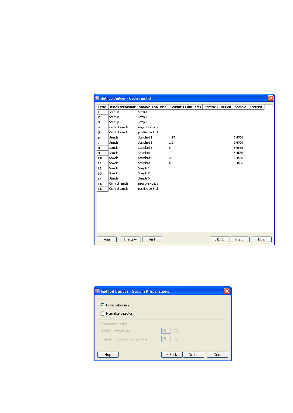
Biacore T200 Software Handbook 28-9768-78 Edition AA 101
Methods 5
5.9.3 Cycle run list
When you have completed the variables table, click Next to view a complete
summary of the cycles that will be performed in the run. This view is for
information only and cannot be edited. Check through the cycle list to confirm
that the variable tables are correctly filled in.
Click Overview to display the method overview (Section 5.3).
5.9.4 System preparations
Choose which preparation steps should be executed before the method starts.

5Methods
5.10 Requirements for assay-specific evaluation
102 Biacore T200 Software Handbook 28-9768-78 Edition AA
System preparations are equivalent to those for wizard-based runs (see
Section 4.2.5). The temperature settings are taken from the first assay step in
the method and cannot be changed here: they are shown for information only.
5.9.5 Rack positions
See Section 4.2.6 for a description of the Rack positions dialog box.
5.9.6 Prepare Run Protocol
See Section 4.2.7 for a description of the Prepare Run Protocol dialog box. Save
the method at this step to include all settings including the Prepare Run protocol
in the saved method.
5.9.7 Starting the run
When the positions are finalized, the sample plate is prepared and loaded into
the instrument and a chip is docked, choose Start Run to start the run. You will
be asked to specify a file name for the results.
5.10 Requirements for assay-specific evaluation
This section describes the requirements and recommendations if assay-specific
evaluation is to be applied to method-based runs.
5.10.1 Concentration analysis
See Chapter 8 for a description of concentration evaluation.
Using calibration
• At least one assay step is required with purpose Calibration and one with
purpose Sample. An assay step with purpose Control Sample is also
required in order to create trend plots for control samples.
• Assay steps Calibration, Sample and Control Sample must be connected
to a cycle type that includes one Sample command. The three assay steps
will normally be connected to the same cycle type.
• Samples in the Calibration step must have concentrations specified in the
variable Conc. At least two different concentrations are required for linear
calibration curves and at least four for 4-parameter fitting.
• Full use of the Calibration trends function (Section 8.2.2) requires
calibration curves run before the first sample cycle and after the last.
• Samples in the Sample step will normally not have specified
concentrations. If concentrations are specified, they will be ignored.

Biacore T200 Software Handbook 28-9768-78 Edition AA 103
Methods 5
Calibration-free
• At least one assay step is required with purpose Sample, connected to a
cycle type that includes one Sample injection with flow rate set to
Variable.
• Each sample must be injected at least twice using different flow rates.
• Evaluation variables D(20°C), MW and Blank must be included for the
Sample injection.
5.10.2 Kinetics/Affinity
See Chapter 9 for a description of kinetics and affinity evaluation.
• At least one assay step is required with purpose Sample, connected to a
cycle type that includes one Sample command.
• Sample concentration must be specified in the variable Conc. If weight-
based units are used, a molecular weight for the analyte must be specified
in the variable MW.
• As a recommendation for multi-cycle kinetics and affinity, there should be
a concentration series with at least four non-zero analyte concentrations
and one zero concentration. At least one of the non-zero concentrations
should be measured in duplicate. Although kinetic and affinity evaluation
can be applied to runs with fewer sensorgrams, the results will generally
be less reliable if these recommendations are not followed.
• Five sample concentrations are recommended for single-cycle kinetics
and affinity, injected in order of increasing concentration. Duplicate cycles
are recommended to ensure robust evaluation. For each determination,
there should be a blank cycle corresponding to the sample cycle, with
buffer replacing the sample for each injection.
5.10.3 Thermodynamics
See Chapter 10 for a description of thermodynamics evaluation.
Thermodynamics evaluation requires that kinetics or affinity (see Section 5.10.2)
is determined at two or more (recommended 5) temperatures.
5.10.4 Affinity in solution
See Chapter 11 for a description of affinity in solution evaluation.
• At least one assay step is required with purpose Calibration and one with
purpose Sample. Both assay steps must be connected to a cycle type that
includes one Sample command. The two assay steps will normally be
connected to the same cycle type.

5Methods
5.10 Requirements for assay-specific evaluation
104 Biacore T200 Software Handbook 28-9768-78 Edition AA
• Samples in the Calibration step must have concentrations specified in the
variable ConcB-calibration. At least two different concentrations are
required for linear calibration curves and at least four for 4-parameter
fitting. These samples should contain only component B.
• Samples in the Sample step must have concentrations specified in the
variables ConcB-fix and ConcA-variable. At least 3 samples with the same
concentration of component B mixed with different concentrations of
component A are required.
5.10.5 Immunogenicity
Evaluation of immunogenicity experiments is described in the separate
Biacore T200 Immunogenicity Handbook.
• For evaluation of specificity confirmation by addition of excess drug,
sample analysis cycles must use the option to mix samples with a
specified solution in the autosampler. For correct evaluation, each sample
should be analyzed twice, once mixed with drug and once with buffer.
• For evaluation of isotyping, isotyping reagents must be injected with the
Enhancement command.
5.10.6 Other requirements
Application of solvent correction (see Section 6.7) requires an assay step with
purpose Solvent Correction, connected to a cycle type that includes at least
four Solvent Correction commands for different solvent concentrations.

Biacore T200 Software Handbook 28-9768-78 Edition AA 105
Evaluation Software

106 Biacore T200 Software Handbook 28-9768-78 Edition AA

Biacore T200 Software Handbook 28-9768-78 Edition AA 107
Evaluation software – general features 6
6 Evaluation software – general features
Biacore T200 Evaluation Software offers general functions for presentation of
results as sensorgrams, report point plots and bar charts, and for evaluation
functions for specific applications such as concentration, kinetics and affinity,
thermodynamics and immunogenicity. There is also a function that corrects for
solvent effects that can sometimes distort the results from analyses with low
molecular weight analytes that give low response levels and require organic
solvents (e.g. dimethyl sulfoxide (DMSO)) to maintain solubility.
This chapter describes the organization of the evaluation software. The various
evaluation functions are described in detail in the following chapters.
6.1 User interface
6.1.1 Organization
The Biacore T200 Evaluation Software screen is divided into four main regions:
•The menu and toolbar provide access to the evaluation functions.
•The Evaluation Explorer at the left of the screen lists the evaluation items
(sensorgrams, plots, bar charts and other result displays) that have been
created in the current session. See below for a description of how to use
the Evaluation Explorer.
Menu and toolbar
Evaluation explorer
Work area
Status bar

6 Evaluation software – general features
6.2 Basic operations
108 Biacore T200 Software Handbook 28-9768-78 Edition AA
•The work area displays the currently open items. Each item is shown in a
separate window that can be moved, resized or closed independently of
the other items.
•The status bar indicates the progress of current operations such as
application of evaluation methods.
6.1.2 The Evaluation Explorer
The Evaluation Explorer lists the sensorgram windows, plots and other
evaluation items in the current evaluation session. Items are organized in
folders according to type. Double-click on a folder to expand or collapse the
folder. Click on an item to display it in the work area. Right click in the explorer
area for options for adding new items: right click on an item for additional
options relating to that item. You can also remove or edit selected items using
the Remove and Edit buttons at the top of the explorer panel.
You can hide the Evaluation Explorer panel to increase the useful size of the
work area by clicking on the pin icon in the explorer title bar. If the panel is
hidden, it will automatically reappear when you move the mouse over the left-
hand edge of the evaluation window.
6.2 Basic operations
6.2.1 Opening files
To open a file in the evaluation software, use the File:Open menu option. You
can open result files from the control software (file extension .blr) and saved
evaluation sessions (file extension .bme). If a file is already open in the software,
opening a new file with File:Open will automatically close the first file. You will
be asked if you want to save the file if any changes have been made.
Opening a file automatically creates and opens an All sensorgrams item, and
creates a number of default plots according to the content of the file.
To open multiple result files in the same session, use the File:Append Result File
option. You can only append result files, not evaluation sessions. Appending a
file to a session will delete all the user-defined evaluation items in the session.
Note: The software does not check that appended result files contain
compatible data. Beware of appending files from different types of run
(e.g. kinetic and concentration analyses) or from the same type of assay
run under different conditions (e.g. concentration assays using different
sensor chips).

Biacore T200 Software Handbook 28-9768-78 Edition AA 109
Evaluation software – general features 6
6.2.2 Printing evaluation results
Choose File:Print to prints a hard-copy of the results. Select the printer to use
and choose the items you wish to print.
6.3 Common display functions
6.3.1 Zooming the display
To zoom a display window, drag with the mouse over the area you want to
enlarge. To restore the previous zoom level, double-click anywhere in the display
window except on the axes or legend, or select Unzoom from the right-click
menu.
Displays are normally rescaled automatically whenever you change the
displayed data. To keep the current zoom setting when data is changed, check
Zoom lock in the display window.
You can also set the display scale with the Scale option from the right-click
menu. The display is not rescaled automatically if the scale has been set to
specified values.
6.3.2 Right-click menus
Right-click in display windows for options relating to the display. The available
options vary according to the type of window, and also depending on whether
you right-click on a point, a curve or elsewhere in the window.

6 Evaluation software – general features
6.3 Common display functions
110 Biacore T200 Software Handbook 28-9768-78 Edition AA
Labels
Displays a label on each point in a plot window, showing cycle number, flow cell
and sample name. (Labels may overlap and be difficult to read if the points in a
plot are closely spaced.)
Caption
Displays a caption in the item window. The displayed caption can have system
defined and user-defined components
Show sensorgram
Displays the sensorgram relating to a point in the plot. This option is only
available when you right-click on a point: the sensorgram is displayed in a
separate window that must be closed before you can continue with the
evaluation.
Exclude cycle/curve/point
Excludes data from the evaluation session. The data that can be excluded
differs according to the type of window. Excluding cycles in sensorgram, plot or
bar chart windows affects all other sensorgram, plot and chart windows
correspondingly: however, application-specific evaluation items that have
already been created are not affected until they are edited and updated. If you
have applied solvent correction and then exclude solvent correction cycles, the
correction remains applied, but the excluded cycles will not be available if you
edit the solvent correction item.

Biacore T200 Software Handbook 28-9768-78 Edition AA 111
Evaluation software – general features 6
Scale
Sets the scale for the display. You can also access this function by double-
clicking on either the x- or y-axis in the display.
Uncheck Auto and enter minimum and maximum values to specify a scale.
Copy graph
Copies the current display as it appears on the screen to the Windows clipboard
as a graphic object, from where it can be pasted into third-party software such
as word-processing or presentation programs.
Copy table
Copies the table data in the current display to the Windows clipboard as tab-
separated text. All rows in the table are copied (including any header row)
regardless of how many rows are visible in the current display. However, in
tables where the columns to be displayed can be selected by the user, only
columns that are currently shown are copied.
Export curves
Exports the curves in the current display to a tab-separated text file, for import
to third-party software. Complete data is exported regardless of the scale
setting of the screen display.
Unzoom
Restores the previous zoom setting.
Gridlines
Shows or hides major and minor gridlines in the display window.
Legend
Shows or hides a legend for the display window. Choose the legend placing from
the dialog box. In sensorgram and plot windows, the legend corresponds to the
Color by setting for the display.

6 Evaluation software – general features
6.4 Predefined evaluation items
112 Biacore T200 Software Handbook 28-9768-78 Edition AA
6.4 Predefined evaluation items
When a result file is opened, a number of evaluation items are created
automatically if the results contain the appropriate cycles and report points.
This section describes the items created for all result files: special items are also
created for certain wizard runs (see Chapter 4).
6.4.1 Sensorgram
An overlay plot of all sensorgrams is created and opened. The sensorgrams are
not aligned, and are colored by assay step.
6.4.2 Plots
Plots are created for most wizards if the appropriate report point is present in
the results. The settings for predefined plots are locked and cannot be edited.
Common predefined plots are listed below. Separate plots will be created if
there are multiple injections with similar report points (for example baseline for
capture and sample injections). The Plot Settings cannot be changed, but the
plot can be modified using the selectors and the Tools menu (see Section 7.2).
Note that changing the selector settings can sometimes defeat the purpose of
the plot.
Baseline: Sample Absolute response for report point baseline
against cycle number.
Baseline: Capture Absolute response for report point
capture_baseline against cycle number.
Baseline: General Absolute response for report point
general_baseline against cycle number.
Binding to reference Relative response for report point stability
against cycle number for the reference flow
cell.
Capture Relative response for report point
capture_level against cycle number for the
capture injection.
Carry-over Relative response for the report point
co_binding against cycle number for the
carry-over injection (only for reference-
subtracted curves).
Controls, binding Relative response for the report point binding
against cycle number for control samples (only
for reference-subtracted curves).

Biacore T200 Software Handbook 28-9768-78 Edition AA 113
Evaluation software – general features 6
6.5 Custom report points
Report points are automatically created for all wizard- and method-based runs,
placed at strategic positions in relation to injections. These report points, and
any other report points that have been created in the Control Software (Section
2.3.3), are not listed in the Custom Report Points dialog and cannot be edited or
deleted in the Evaluation Software.
Choose Tools:Custom Report Points to add and edit custom report points.
Controls, stability Relative response for the report point stability
against cycle number for control samples.
Binding levels Relative response for the report point binding
against cycle number for samples (only for
reference-subtracted curves).
Binding stability Relative response for the report point stability
against cycle number for samples.
Binding to reference,
enhancement
Relative response for report point
enhance_level against cycle number for
enhancement injections on the reference
surface.
Enhancement Relative response for the report point
enhance_level against cycle number for
enhancement injections on the active surface.

6 Evaluation software – general features
6.5 Custom report points
114 Biacore T200 Software Handbook 28-9768-78 Edition AA
6.5.1 Adding report points
Click Add to add a new report point.
Enter a name for the report point (maximum 30 characters) in the Id field. The
report point name must be unique within an evaluation session.
Enter a value between 1 and 35 for the Window. Preset values of 5, 10 and 15
seconds are provided for convenience: a window of 5 seconds is recommended
for most purposes. The response value for the report point is the average
response over the window, with the report point time at the center of the
window.
Use the settings under Position the report point to define where the report
point will be placed. Report points are placed a specified number of seconds
before or after the beginning or end of injections or the beginning or end of the
cycle.
Notes: Do not position report points far away from events so that they lose their
relevance to the event, or so close to an event so that the report point
window overlaps the event itself.
You cannot define a report point with settings that would place part of the
window outside the time limits of the sensorgram.
Check Calculate response relative to report point and select the required
report point if you want to calculate the responses at the custom report point
relative to another report point. If the box is not checked, the closest preceding
baseline report point will be used for calculating relative response values.

Biacore T200 Software Handbook 28-9768-78 Edition AA 115
Evaluation software – general features 6
You can apply custom report points either to cycles with selected assay step
purposes or to cycles selected by cycle number. Choose the appropriate option
and check the assay step purpose(s) or cycles to which the report point should
apply.
Note: If you append a result file to the evaluation session after creating custom
report points, the custom report points are retained but they are not
applied to sensorgrams in the appended file.
6.5.2 Editing and deleting report points
Select a report point in the list in the Custom Report Points dialog and click Edit
to edit the report point definition or Delete to delete the report point.
Notes: All user-defined evaluation items are deleted from the session when
custom report points are edited or deleted, since changes to the report
point definitions may affect existing evaluation items. You will be warned
when this occurs. To avoid losing work, save your evaluation session
before editing or deleting custom report points.
If you delete a custom report point that is used as baseline for other report
points, the relative response can no longer be calculated for the latter
points. You will be warned if this situation arises.
6.6 Keywords
Keywords are assigned to cycles when the run is performed, and are then used
for identification and evaluation purposes. Keywords are created automatically
for wizard-based runs and may be defined in the method for method-based
runs, and include:
• automatically generated identifiers such as cycle number or assay step
purpose,
• method variables and predefined evaluation variables such as sample
name, concentration and molecular weight,
• user-defined variables (see Section 5.6.2).
You can add and remove user-defined keywords in the evaluation software, and
edit the contents of certain keywords. Choose Tools:Keyword Table to open the
keyword table. When you save changes to the keyword table, all user-defined
items in the evaluation session will be deleted. Save the session before editing
the keyword table if you do not want to lose your work. Click Cancel in the
Keyword Table dialog to close the dialog without applying changes and
deleting user-defined evaluation items.

6 Evaluation software – general features
6.6 Keywords
116 Biacore T200 Software Handbook 28-9768-78 Edition AA
To simplify management of the keyword table, you can sort and filter the table
display:
• Click on a column header to sort the table by the contents of that column.
• Click in the filter row (directly below the column header) and select a value
to display only rows with that value for the chosen column. Click Reset All
Filters to restore all filters to the [All] setting.
To change a keyword value, simply enter the new value in the appropriate cell.
Values for some system-generated keywords (such as Assay Step Purpose) are
chosen from a predefined list of values: the list is displayed when you click in
such a cell.
To change the units for concentration keywords, choose a new unit from the
Concentration Unit list. This changes the unit but not the numerical value of the
keyword. For example, a concentration entered as 10 µM will become 10 mM if
you change the concentration unit to mM. If the evaluation session includes
data from multiple files, a table of concentration units for the different files is
displayed. Make sure that the unit is the same for all files if data are to be
evaluated together.
Note: The concentration unit affects only predefined concentration keywords.
Numerical user-defined keywords are simply numbers, and will not be re-
interpreted when you change the concentration unit even if they are
intended to hold concentration information.
Click Add Keyword to create a new keyword in the table. You can choose
between predefined keywords and user-defined keywords (see Section 5.6.2). If
there are multiple Sample or General commands in the method from which the
data is obtained (see Section 5.6.1), specify the command to which the new
keyword should apply.

Biacore T200 Software Handbook 28-9768-78 Edition AA 117
Evaluation software – general features 6
Enter the required keyword values in the empty column that is created for the
new keyword.
To rename or delete a keyword, click the appropriate button, then select the
keyword in the dialog box. You cannot remove system-generated keywords
such as file number or cycle number, or keywords derived from method
variables such as sample name.
6.7 Solvent correction
6.7.1 Background
Solvent correction adjusts reference-subtracted responses for small artefacts
that can be introduced by variations in the bulk refractive index between
samples. The correction is only relevant when variations in the bulk refractive
index are of the same order of magnitude as the response: this situation arises
commonly in work with small organic analytes that give intrinsically low
response values and that often require organic solvents such as dimethyl
sulfoxide (DMSO) to maintain solubility.
The need for solvent correction arises because subtraction of the reference
response does not exactly eliminate the contribution of the bulk solution to the
measured response. Bulk solution is excluded from the volume occupied by
ligand on the active surface, so that the bulk contribution to the response on the
active surface is slightly smaller than that on the reference surface (Figure 6-1).

6 Evaluation software – general features
6.7 Solvent correction
118 Biacore T200 Software Handbook 28-9768-78 Edition AA
Figure 6-1. Bulk solution is excluded from the volume occupied by ligand molecules on the
ligand surface, so the bulk contribution to the relative response is smaller than on the
reference surface.
As long as the refractive index of the samples is constant, this excluded volume
effect introduces a constant error in reference subtraction which may be
ignored for practical purposes. However, if the refractive index of the samples
varies, the magnitude of the excluded volume effect will also vary.
Organic solvents like DMSO often give a high bulk response (addition of 1%
DMSO gives a bulk response of about 1200 RU), so that small variations in the
DMSO content lead to significant variations in the bulk response between
samples. Such variations are unavoidable in the preparation of diverse samples
such as drug candidates for screening applications. The solvent correction
procedure corrects for the variations arising from the excluded volume effect in
these cases.
A more detailed description of solvent correction background and procedures
may be obtained from GE Healthcare.
6.7.2 When solvent correction should be used
It is important to bear in mind that solvent correction is only relevant when
• the expected analyte responses are low,
• the ligand is a macromolecule immobilized at a high density (typically
5,000 RU or more – lower ligand densities lead to excluded volume effects
that are too small to merit correction),
• the bulk response is subject to variations between samples of at least the
same order of magnitude as the measured binding response.
Solvent correction should not be applied in situations that do not meet all three
of these criteria. Attempts to use solvent correction in other circumstances may
introduce errors that are larger than the solvent effects that the procedure is
intended to correct.
Response on
reference surface
Response on
ligand surface
Excluded volume effect
Ligand surface
Reference surface

Biacore T200 Software Handbook 28-9768-78 Edition AA 119
Evaluation software – general features 6
6.7.3 How solvent correction works
Solvent correction factors are determined by injecting a series of blank samples
containing a range of solvent concentrations over the active and reference
surfaces, and plotting the difference in relative response between the surfaces
as a function of the relative response on the reference surface. Each sample
measurement is then corrected by a factor obtained by measuring the relative
response on the reference surface and reading the corresponding difference
between active and reference surfaces from the correction curve (Figure 6-2).
Figure 6-2. The principle of solvent correction. 1. The sensorgram from the reference flow
cell shows a bulk displacement (-150 RU in the illustration) during sample injection because
the sample and running buffer are not exactly matched. 2. From the solvent correction
curve, a displacement of –150 RU in the reference sensorgram corresponds to a solvent
error of +5 RU in the reference-subtracted sensorgram. 3. The reference-subtracted
sensorgram is corrected by subtracting the solvent error. This procedure is applied to every
point during sample injection.
Solvent correction is applied only to response levels during sample injection,
since the correction adjusts for differences in the bulk refractive index of the
samples compared with running buffer. Solvent correction is meaningless when
buffer is flowing over the surface before and after the sample injection.
6.7.4 Applying solvent correction
To apply solvent correction, choose Add solvent correction from the Evaluation
menu. In order to apply solvent correction, the run must include solvent
correction cycles (see Section 5.6.1).

6 Evaluation software – general features
6.7 Solvent correction
120 Biacore T200 Software Handbook 28-9768-78 Edition AA
The left-hand panel of this dialog lists the solvent correction curves in the run,
and the corresponding curves are shown in the right-hand panel. For each
solvent correction cycle, there is one correction curve for each set of reference-
subtracted sensorgrams. All cycles are shown by default in an overlay plot.
Select specific rows in the cycle list to display the corresponding solvent
correction curves. Clear the checkmark in the Included box to exclude cycles
from the correction calculation. You must include at least one solvent correction
cycle for each curve. Sample responses are corrected according to the curve
obtained from the nearest preceding correction cycle in the run. If there is no
preceding correction cycle, the nearest following cycle is used.
Examine the curves for fitting to the experimental points. Right-click on outlying
points to exclude either the single point from the curve fit or the whole
correction cycle from the correction process. Statistical fitting parameters (chi-
squared) are shown for each correction curve in the cycles list. Right-click on a
point or curve in the right panel and choose Show sensorgrams if you want to
examine the sensorgrams from solvent correction cycles as an aid in judging the
quality of the data.
The solvent correction curve is fitted to the experimental points using a second-
degree equation. Beware of applying solvent correction if the correction curve
does not fit the experimental points closely. Scatter in the correction points
indicates that the measurements are not reliable, and applying correction
derived from such curves can distort the measured responses unnecessarily.
For reliable solvent correction, the chi-squared value should be less than 2 RU.
Note: In judging the quality of the solvent correction data, take note of the y-axis
scale in the display. The curves are automatically scaled to fit the window.

Biacore T200 Software Handbook 28-9768-78 Edition AA 121
Evaluation software – general features 6
If the range of solvent correction is small (as in the illustration above),
points may appear to scatter around the fitted curve without necessarily
indicating poor curve quality.
The shape and slope of the solvent correction curve (even the direction of slope)
may vary between measurements on different occasions. This is normal and the
shape of the curve should not be taken as an indicator of curve quality.
The range of report point values that are candidates for solvent correction in the
assay data is indicated by vertical red lines in the window. If report points lie
outside the correction range, these values cannot be properly corrected. Some
small extrapolation of the correction plots may be permissible. Use the
Extrapolate button to extend the correction range. The shape of the solvent
correction plots is however not fully predictable, and extrapolation over more
than about 10% of the range of the reference values is dangerous.
Click OK to apply the solvent correction. Correction will be applied to the sample
and carry-over injection phase(s) of all sensorgrams. Any data points that lie
outside the correction range will be discarded and the corresponding
sensorgram will contain gaps corresponding to the invalid data.
Note: In assays where the temperature is varied during the run, such as
thermodynamics assays, you should make sure that there is a solvent
correction curve included at the start of each temperature series.
Correction will only be applied to sample measurements made at the
same temperature as the correction curve.
6.8 Evaluation methods
Evaluation methods allow you to save the definitions of all evaluation items
(except Thermodynamics) in an evaluation session, and apply them
automatically to the same or different result files or evaluation sessions. Use this
feature to apply standardized evaluation procedures to different result files, or
to re-create an evaluation session after operations that delete user-defined
items such as changes made in the custom report points or keyword table (see
Sections 6.5 and 6.6).
6.8.1 Creating evaluation methods
To create an evaluation method, choose File:Save Evaluation Method As and
specify a file name and location. The method is saved with file extension
.evalmethod.
An evaluation method may only contain one definition of a kinetics/affinity
evaluation item. If there are more than one item in the evaluation session, or if
an item contains more than one fitting, you will be asked to choose which item
should be represented in the method.

6 Evaluation software – general features
6.8 Evaluation methods
122 Biacore T200 Software Handbook 28-9768-78 Edition AA
Click Skip to create the method with no kinetics/affinity item included.
Calibration-free concentration analysis items that have different fitting ranges
for different samples (Section 8.3) and kinetic/affinity items that use data sets
with multiple R
max
(Section 9.2.2) cannot be saved in evaluation methods.
6.8.2 Applying evaluation methods
To apply an evaluation method to the contents of an evaluation session, choose
File:Apply Evaluation Method and choose the method. A preview of the method
is shown so that you can check the method contents.
Click Apply to apply the method. Items in the method will be created where
possible. Items that cannot be created will be reported in a dialog box.

Biacore T200 Software Handbook 28-9768-78 Edition AA 123
Data presentation tools 7
7 Data presentation tools
This chapter describes the tools available for presentation and examination of
the data in a result set. These tools comprise:
• Sensorgram display, with facilities for aligning sensorgrams in overlay
plots.
• Plot tool for displaying and ranking response values.
• Bar chart for displaying response values.
• A report point table for listing numerical values associated with report
points.
7.1 Sensorgram items
Sensorgram items display sensorgrams from one or more cycles in the results.
A sensorgram item showing all sensorgrams for the first reference-subtracted
curve in the results (or first active curve if reference subtraction is not used) is
created automatically when the result file is opened. You can change the display
settings in this item, or create additional sensorgram items if required. Click
Sensorgram in the toolbar or choose Add sensorgram from the Evaluation
menu to add a new sensorgram item.
Hold the cursor over a sensorgram to display a tool tip identifying that particular
curve. The sensorgram coloring can be changed if desired with the Tools:Color
by option.
The following sections describe display functions specific to sensorgram items.
General display functions are described in Section 6.3.

7 Data presentation tools
7.1 Sensorgram items
124 Biacore T200 Software Handbook 28-9768-78 Edition AA
7.1.1 Selecting sensorgrams for display
The selector bar at the top of the window controls which sensorgrams will be
displayed.
• Curve name lists the type of sensorgram (active, reference, reference
subtracted and solvent corrected where applicable).
• Assay Step Purpose filters the sensorgram according to the assay step
purpose.
• Cycle lists all the cycles in the result set. When multiple files are open,
cycles are identified with two numbers, one for the file in the result set and
one for the cycle within the file (thus cycle 1-10 is the 10
th
cycle in the first
file added to the result set; cycle 2-4 is the 4
th
cycle in the second file and
so on).
For each display controller, click the browse buttons to browse backwards or
forwards through the list, one item at a time.
Click the selector button to open the list for selecting one or more items. Drag
with the mouse or use shift-click to select contiguous multiple items. Use
control-click to select non-contiguous multiple items. To accept a selection, click
anywhere outside the list or press Enter.
7.1.2 Removing data
To remove data from the display, mark the section to be removed by dragging
with the right mouse button, then choose Cut from the right-click menu. The
data will be removed from the current sensorgram display item only; no other
windows or evaluation items will be affected. This function can be useful for
removing injections with high bulk contributions (such as regeneration
injections) or other visual disturbances from the display.
Choose Undo Cut from the right-click menu to restore the removed data.

Biacore T200 Software Handbook 28-9768-78 Edition AA 125
Data presentation tools 7
7.1.3 Sensorgram adjustment
Choose Sensorgram adjustment under the Tools button for options for aligning
and adjusting the sensorgram display. For curve alignment, sensorgrams that
do not include the chosen reference point for alignment will not be shown.
Sensorgram adjustment only affects the display in the current sensorgram item.
X-adjustment
Choose to set the zero time point to either a report point or an injection event. If
this setting is Off, the zero time point will be at the beginning of the cycle.
Y-adjustment
Choose to set the zero response point to either a report point or an injection
event. If this setting is Off, the actual response values will be shown.
If you check Enable Second Y-Adjustment, you can select a report point or
injection event where the response value will be set to 100. Each sensorgram will
then be normalized separately to the first and second adjustment point, so that
all sensorgrams will have values of 0 and 100 at these points regardless of the
original response levels. This can help in comparing the shapes of sensorgrams
independently of their response levels, or in adjusting response levels that are
dependent on others (e.g. adjusting analyte response for varying capture levels,
by adjusting the baseline to 0 and the capture level to 100).

7 Data presentation tools
7.1 Sensorgram items
126 Biacore T200 Software Handbook 28-9768-78 Edition AA
Blank subtraction
Check Enable Blank Subtraction and choose a curve to be used as the blank to
subtract one sensorgram from all others in the display. Use this feature to
eliminate systematic disturbances in sensorgrams that are not removed by
reference subtraction. Blank subtraction only affects the current sensorgram
window: other evaluation items are not affected.
Note: Subtracting a blank sensorgram is not the same as using reference-
subtracted data. Reference subtraction gives the difference between
active and reference values for each cycle separately for each curve,
whereas blank subtraction subtracts one curve from all others in the
result set.
7.1.4 Markers
You can choose to display markers and/or labels for report points and events in
the cycle with the Report points and Event markers options respectively under
the Tools button. Report points are displayed on the curve and event markers
on the x-axis.

Biacore T200 Software Handbook 28-9768-78 Edition AA 127
Data presentation tools 7
7.2 Plot items
Plot items display report point values plotted against either variables or other
report point values in the same cycle. Curves can be fitted to points using linear
or 4-parameter fitting functions. Ranking borders can be added to plot items to
classify response levels into groups such as high, medium and low responses.
To create a plot item, click Plot in the toolbar or choose Add Plot from the
Evaluation menu. Enter a name for the plot, choose the parameters that define
the plot and click Finish. Cycles that do not contain the selected report point will
not be represented in the plot.
Response type may be response (absolute or relative response, or relative
response adjusted for molecular weight if the keyword MW is defined) or
sensorgram slope at the selected report point. Adjustment for molecular weight
is performed by dividing the response in RU by the molecular weight in Da.
Points for which the molecular weight value is zero or missing are omitted from
the plot.
Variables may be numerical (e.g. molecular weight or concentration) or non-
numerical (e.g. sample name or assay step purpose).
The plot will be created with default display settings, with a graphical
representation at the left and a table of x-and y-values at the right. Tool tips
identify the data points (place the cursor on a point for a couple of seconds to
display the tool tip).

7 Data presentation tools
7.2 Plot items
128 Biacore T200 Software Handbook 28-9768-78 Edition AA
Right-click on the plot item in the evaluation explorer and choose Rename to
change the plot name.
7.2.1 Selector functions
The selector bar at the top of the window controls which points will be displayed.
• Curve name lists the type of sensorgram from which the points are taken
(active, reference, reference subtracted and solvent corrected where
applicable).
• Assay Step Purpose filters the points according to the assay step purpose.
• The third selector lists the variable values represented on the x-axis. (This
option is not available for plots of report point against report point.)
Selection operates in the same way as in the sensorgram window (Section 7.1.1).
Other general display functions are described in Section 6.3.

Biacore T200 Software Handbook 28-9768-78 Edition AA 129
Data presentation tools 7
7.2.2 Table functions
The table to the right of the plot area lists values for the points in the plot.
Excluded points are shown struck out in red text. You can exclude or include
cycles from the right-click menu in the table area, in the same way as from the
right-click menu in the plot. The table also allows you to exclude or include
multiple cycles in a single operation.
Select rows in the table to highlight the corresponding points in the plot. If you
select a single row, the highlight is augmented with lines drawn to the plot axes:
By default, the table shows x- and y-values and is sorted in ascending order of
x-values. Click on the header row to select the sort value and to change the sort
order. Sorting the table does not have any effect on the plot display.
Choose Tools:Table columns to select columns that will be displayed in the
table. You can also change the order in which columns will be displayed using
the Move up and Move down buttons (the top of the column list represents the
left-hand column in the table).

7 Data presentation tools
7.2 Plot items
130 Biacore T200 Software Handbook 28-9768-78 Edition AA
7.2.3 Sorting the plot
Plots of report point values against variables can be sorted in order of ascending
or descending y-axis value, regardless of the variable chosen for the x-axis. A
sorted plot can be useful for example in visualizing the frequency of different
levels of response, which may be more difficult to see if the levels are scattered
more or less randomly with respect to the variable parameter defined for the
x-axis. Choose Sort:Ascending or Descending under the Tools button to sort
the plot. Sorting the plot also sorts the rows in the table, although the table can
be sorted independently of the plot by clicking in the table column header
(Section 7.2.2).
Note: By default, the table associated with a sorted plot retains a column
labeled X-Value. This is the value of the variable originally defined for the
plot, and does not correspond to the x-axis as displayed in the sorted plot.
Choose Sort:As Defined to restore the x-axis to the originally defined variable
value.
Plots of one report point against another cannot be sorted.
7.2.4 Fitting curves to points
Choose Curve Fitting under the Tools button to fit lines to the points in the plot.
using either linear or curved (4-parameter) fitting functions. If Fit by color is
checked, each color will be fitted to an independent line. If this option is not
checked, all points derived from the same curve will be fitted to a single line. The
numerical fitting results are displayed in an extra panel below the plot. Choose
Curve Fitting:Curve parameters under the Tools button to toggle display of this
extra panel.

Biacore T200 Software Handbook 28-9768-78 Edition AA 131
Data presentation tools 7
For linear fitting, the points are fitted to the equation
y = slope * x + intercept
The equation for a 4-parameter fit is
The closeness of fit is reported for linear fitting as the coefficient of
determination R
2
and for 4-parameter fitting as the chi-squared value (see
Section 9.7.1).
Curve fitting cannot be applied to plots that have been sorted.
where y and x are the plot coordinates
R
hi
and R
lo
are fitting parameters that correspond to the maximum and
minimum response levels respectively
A
1
and A
2
are additional fitting parameters
y R
hi
R
hi
R
lo
–
1
x
A
1
----- -
⎝⎠
⎛⎞
A
2
+
--------------------------
–=

7 Data presentation tools
7.2 Plot items
132 Biacore T200 Software Handbook 28-9768-78 Edition AA
7.2.5 Adjusting plots for controls
Plots can be adjusted for systematic changes in response during the course of
the assay, such as progressive loss of binding capacity resulting from harsh
regeneration conditions. Adjustment is calculated from the response values
obtained for control samples analyzed at intervals during the assay.
Adjustment for controls cannot be applied to plots of one report point against
another.
To apply this adjustment, choose Adjustment for controls from the Tools menu
in the plot window. Check Use adjustment for controls and select the sample to
use as a positive control. You can also select a sample for the negative control.
Select whether the adjustment should be made using a linear or polynomial
(second degree) fitting function. The display panels in the dialog show a plot of
the response against cycle number before and after adjustment. Click OK to
apply the adjustment.
Adjustment normalizes the sample responses relative to the positive and
negative control levels as follows:
• Curves are fitted to the control sample responses for positive and (if used)
negative controls. The Linear option fits the points to a function with the
form y=ax+b (where a and b are constants). Polynomial fits the points
to a second-degree function with the form y=ax
2
+bx+c (where a, b and
c are constants). If no sample is chosen as a negative control, 0 RU is used
as the negative control response.
• The fitted line(s) are transformed to straight horizontal lines with values
100 for the positive control and 0 for the negative control.

Biacore T200 Software Handbook 28-9768-78 Edition AA 133
Data presentation tools 7
• The transformation used to create straight horizontal lines for the control
points is applied to all points in the plot (including the actual control
sample responses) so that each point retains the same position relative to
the positive and negative controls before and after adjustment.
Adjustment for controls cannot be applied in regions where the positive control
curve lies below the negative control curve (or below the x-axis if no negative
control is selected). Any points that lie in such regions will be excluded from the
adjusted plot.
Adjustment for controls applies only to the current plot and does not affect any
other evaluation item.
Note: Beware of using a polynomial fitting function with less than 4 control
samples. The parabolic curve created by the function can deviate greatly
from the points, leading to adjustment that does not reflect the drift in the
control responses (Figure 7-1).
Figure 7-1. Polynomial function fitted to 3 control points (highlighted) with the resultant
adjustment for controls.
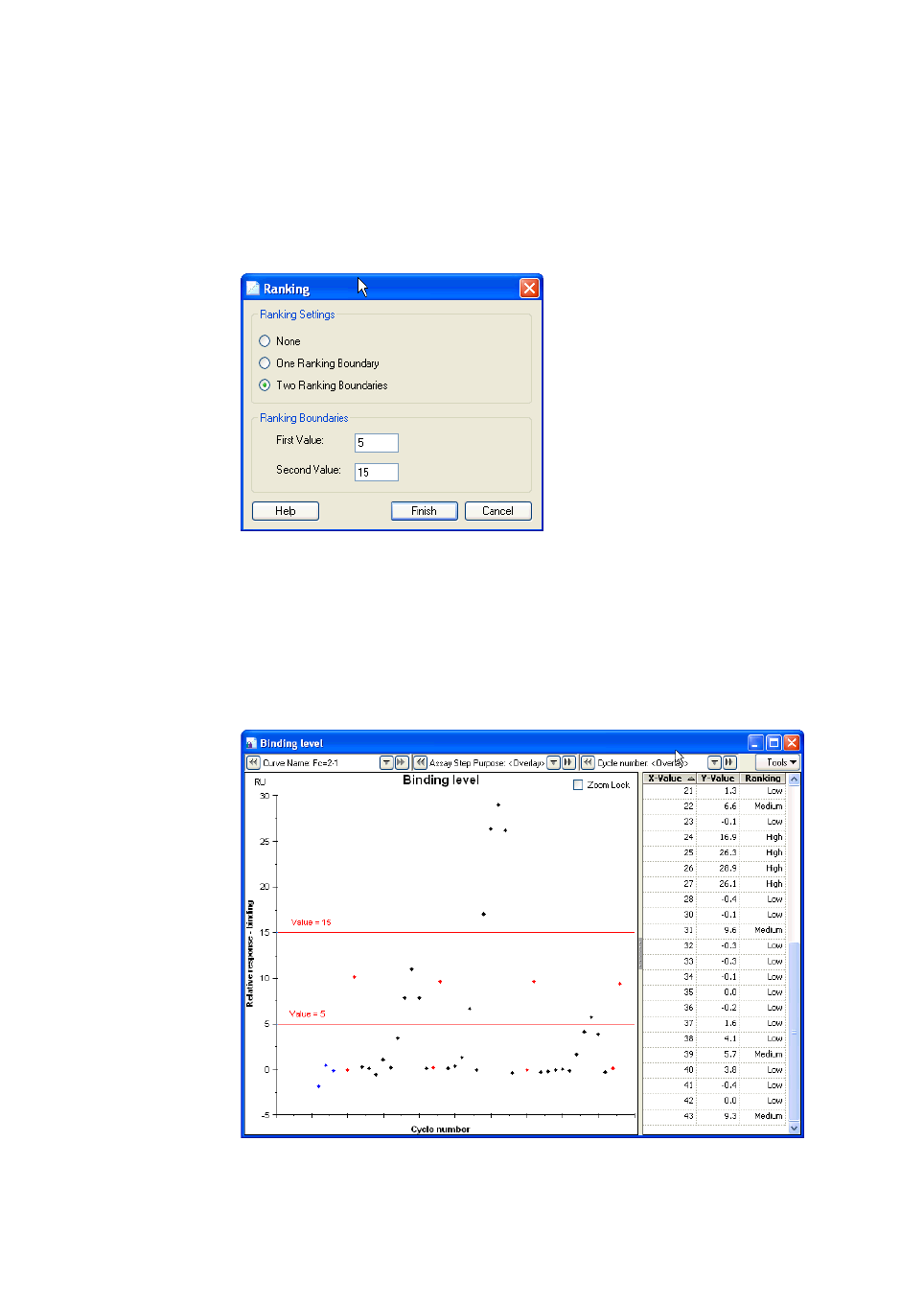
7 Data presentation tools
7.2 Plot items
134 Biacore T200 Software Handbook 28-9768-78 Edition AA
7.2.6 Ranking
Choose Ranking under the Tools button to add ranking boundaries to the plot.
You can add one or two boundaries, classifying the plot points as Low/High or
Low/Medium/High. The boundary values are specified in RU.
Boundaries are shown as horizontal red lines in the plot, labeled with the
boundary value. The classification of the points is recorded in the table. Ranking
results are independent for each plot item.
Note: Editing the definition of a plot does not affect ranking boundaries. If you
for example change the y-axis parameter of a ranked plot from relative
response to absolute response, you will need to revise the placing of the
ranking boundaries if the ranking is to remain meaningful.

Biacore T200 Software Handbook 28-9768-78 Edition AA 135
Data presentation tools 7
7.3 Bar chart items
Bar charts display report point data plotted against cycle number. Unlike plots,
bar charts can display multiple report points in the same chart, and can group
the display in various ways.
To create a bar chart, click Bar Chart in the toolbar or choose Add Bar Chart
from the Evaluation menu. The chart is created directly. Numerical values on
which the chart is based are listed on the Table tab.
7.3.1 Selector functions
Select the curves to display in the lower left hand panel, cycles in the center
panel and report points in the right-hand panel. In each panel you can select
multiple rows by dragging with the mouse or using Shift-click for contiguous
rows or Control-click for non-contiguous rows. Click on the column header in the
table of cycles in the center panel to sort the table by the contents of the
column, to simplify selection of rows according to the required criteria.
Select whether to display relative or absolute response values in the Response
field. This selection applies to all report points shown in the chart. Points for
which the selection is invalid are not shown (for example, the report point
baseline will normally not be shown on a bar chart of relative response).

7 Data presentation tools
7.4 Report point table
136 Biacore T200 Software Handbook 28-9768-78 Edition AA
7.3.2 Display options
Drag with the mouse to zoom the bar chart display. Double-click to restore the
original scaling.
Use the Tools menu to determine how the bar chart is organized and displayed:
Group by
You can group bars in the chart by various parameters such as curve, cycle,
report point or sample name. Groups are separated by vertical lines in the chart.
Grouping is most useful when you have multiple selections in more than one
selection panel: the examples below illustrate bar charts showing two report
points, grouped by cycle (left) and by report point (right).
Color by
Select a parameter in the Color by list to color the bars in the chart according
to the parameter value. A Color key will be added to the table in the appropriate
panel.
Show column labels
Use this option to display labels identifying the bars in the chart. The bars are
also identified by tool tips, regardless of whether labels are displayed or not.
7.4 Report point table
Report points are automatically created for all wizard- and method-based runs,
placed at strategic positions in relation to injections. See Section 6.5 for details
of how to add custom report points.
7.4.1 Displaying the report point table
The report point table lists numerical values for all report points in the current
result set. The report point table is created automatically as an evaluation item.
Each evaluation session can only have one report point table item: the table is
updated automatically if you add custom report points or apply solvent
correction.
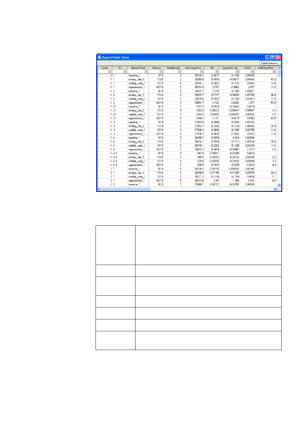
Biacore T200 Software Handbook 28-9768-78 Edition AA 137
Data presentation tools 7
The contents of the report point table cannot be edited.
The following columns can be represented in the report point table. Click the
Table Columns button to choose which columns to display.
File File number. This column is only shown when the
evaluation session includes more than one file, the cycle
number is prefixed with a file number. Choose
File:Properties to display the mapping of source files to file
numbers.
Cycle Cycle number within the file.
Fc The curve to which the report point applies, identified as
the flow cell.
Report point Report point id.
Time (s) Report point time in seconds from the start of the cycle.
Window (s) Report point time window in seconds.
AbsResp (RU) Absolute response in RU, calculated as the mean value
over the time window.

7 Data presentation tools
7.4 Report point table
138 Biacore T200 Software Handbook 28-9768-78 Edition AA
Sorting and filtering the report point table
The report point table can be sorted by any column in ascending or descending
order for any column. Click in the header for a column to sort the table by that
column. Each click in the same header toggles the sort order.
SD Standard deviation of data points in the time window,
calculated as
where n = number of points
and y = response in RU
Slope (RU/s) Slope during time window in RU s
-1
, calculated as
LRSD Alignment of slope to a straight line (regression coefficient),
calculated as
where
Baseline Yes for report points defined as baseline. Otherwise No.
RelResp (RU) Relative response (difference in absolute response from the
baseline) in RU. #N/A if no baseline has been set.
AssayStep
Purpose
CycleType
Identifiers for the cycles, set explicitly in methods (see
Chapter 5) and automatically in wizards.
Keywords One column is created for each keyword in the data.
SD
1
n1–()
-----------------
yy–()
2
∑
=
slope
yy–()xx–()
∑
xx–()
2
∑
----------------------------------------
=
LRSD
Q
0
n2–()
-----------------=
Q
0
yy–()
2
yy–()xx–()
∑
()
2
xx–()
2
∑
----------------------------------------------- -
–
∑
=
Header row
Filter row

Biacore T200 Software Handbook 28-9768-78 Edition AA 139
Data presentation tools 7
The second row in the report point table contains a filter setting for each
column. All values will be included if the filter setting is blank. To apply a filter,
click on the setting and select a value from the list. The value will be shown in
the filter setting and only rows in the table that contain the value in the selected
column will be displayed. You can apply multiple filters to the table at the same
time. To remove a filter, choose All from the list of column values in the filter
setting.
Copying report point table contents
To copy the selected contents of the report point table, select cells by dragging
with the mouse and press Ctrl-C or choose Copy from the right-click menu.
Choose Copy Table to copy the whole table. The contents will be copied in tab-
separated text format to the Windows clipboard, and can be pasted from there
into other programs. All selected cells will be copied, including header cells and
filter settings.

7 Data presentation tools
7.4 Report point table
140 Biacore T200 Software Handbook 28-9768-78 Edition AA

Biacore T200 Software Handbook 28-9768-78 Edition AA 141
Concentration analysis 8
8 Concentration analysis
Biacore T200 software supports two approaches to concentration analysis:
• Using a calibration curve determined by measurement of known samples
(referred to as calibrated measurements).
• Calibration-free measurements that rely on the relationship between the
analyte concentration and the rate of mass transfer of analyte to the
sensor surface.
Principles and experimental practice for concentration measurements are
described in the Biacore Concentration Analysis Handbook.
8.1 Requirements for concentration evaluation
8.1.1 Calibrated measurements
In order to evaluate concentration analysis using a calibration curve, the run
must include at least one calibration curve and unknown sample injections
must have the appropriate properties and keywords. For wizard-based runs, the
conditions are met automatically when the Concentration Analysis wizard is
used. For method-based runs, the method must be constructed as described in
Section 5.10.1: if necessary, the keyword table can be edited so that the
conditions are met in full (see Section 6.6). Note however that the command
name for the sample injection cannot be edited in the keyword table. Refer to
Chapter 5 for details of how to construct methods in Method Builder.
Unknown samples may be evaluated in three ways:
• Based on the nearest preceding measured calibration curve, or the
nearest following curve if there is none preceding.
• Based on a single calibration curve constructed as an average of all
measured curves.
• Based on individual calibration curves constructed for each separate
cycle, using a calibration trend plot to interpolate calibration data between
the measured points. This option is useful if the calibration responses show
a steady drift during the course of the assay.
8.1.2 Calibration-free measurements
Runs for calibration-free concentration analysis require a minimum of two
cycles for each sample, run at different flow rates. Blank cycles for each flow
rate are recommended. Both samples and blanks must be injected with a
command of type Sample (see Section 5.6.1). No calibration standards are
required.

8 Concentration analysis
8.2 Evaluating calibrated concentration analyses
142 Biacore T200 Software Handbook 28-9768-78 Edition AA
Correct values for the diffusion coefficient D at 20°C and the molecular weight
MW must be provided. These values are normally provided when the run is set
up in the Control Software, but can be added or edited in the keyword table in
the Evaluation Software.
8.2 Evaluating calibrated concentration analyses
To evaluate a concentration analysis run, open the run and choose
Concentration Analysis:Using calibration from the evaluation toolbar, or
choose Add Concentration Analysis:Using calibration from the Evaluation
menu. The evaluation dialog is divided into three tabs, for calibration curves,
control samples and unknown samples respectively. Choose the appropriate
settings for the calibration curves and click Finish to complete the evaluation.
8.2.1 Calibration curves
A calibration curve is constructed from the cycles in each calibration step. If two
calibration steps are run in direct succession so that there are no other cycles
between the steps, they will be combined in a single calibration curve.
Settings on the Calibration tab define the report point and fitting function that
are used to create the calibration curve. The settings apply to all calibration
curves in the evaluation. Choose the settings appropriate for your analysis:

Biacore T200 Software Handbook 28-9768-78 Edition AA 143
Concentration analysis 8
Check Use average calibration curve to use one average curve constructed
from all calibration points in the run.
Check Use calibration trends to create individual calibration curves for each
cycle in the assay by interpolation between the actual measured calibration
curves. See Section 8.2.2 for details of calibration trends.
The left-hand panel lists the details of the calibration curve data, with
concentration and response or slope values for all calibration points. The
Calc. Conc. column lists the concentration corresponding to the actual
response value as determined from the fitted calibration curve. Select a row in
the table to highlight the corresponding point on the calibration curve or vice
versa. Fitting parameters are shown at the bottom of the left-hand panel when
a single calibration curve is displayed.
The calibration curves are shown in the right-hand panel. Each calibration curve
is constructed from the cycles in an assay step with the purpose Calibration.
Right-click on a curve or calibration point for options for excluding calibration
curves or single cycles from the evaluation, and for displaying sensorgrams
corresponding to individual calibration cycles. Excluded cycles are shown as
open symbols and are marked in the left-hand panel with red strikethrough text.
If you exclude a calibration curve and then re-include sufficient points to allow
a new curve to be fitted, the curve will still be excluded but will be shown as a
broken line.
Flow cell Concentration analysis may be performed without a reference
cell, since the unknown samples are determined by direct
reference to a calibration curve obtained under the same
conditions. If a reference cell is included in the flow path for
the run, the reference-subtracted curve may however be
selected if desired.
Report point Response levels for concentration analysis (relative response)
are normally taken from a report point shortly after the end of
the sample injection, to avoid contributions from the bulk
refractive index of the sample. For analyses based on the rate
of binding (report point slope), a report point early in the
sample injection is normally used.
Response type Choose between relative response and slope.

8 Concentration analysis
8.2 Evaluating calibrated concentration analyses
144 Biacore T200 Software Handbook 28-9768-78 Edition AA
You can choose the curve to display from the list at the top of the panel. The
options differ according to how the calibration curves are used:
•For Use preceding calibration curve, the panel shows one calibration
curve by default. Individual curves multiple curves can be selected from
the list.
•For Use average calibration curves, the panel shows all calibration points
with a single average curve.
•For Use calibration trends, the panel shows all measured calibration
curves in an overlay plot.
Note: The sample name entered for the calibration samples is used only as a
title for the calibration curve. For wizard-based runs, the sample name
will be the same for all calibration cycles, but different names can be
introduced either in method-based runs or by editing the keyword table.
If the points in a calibration curve have different sample names, all points
will still be used and the title will be shown as Mixed analytes.
Choose the Fitting Function for the calibration curve from the option above the
curve panel. Linear and 4-parameter functions and provided with the software,
and custom models can be defined if required (Section 8.2.5). The 4-parameter
function is a general fitting function for continuous curves, and is recommended
for most purposes. Use a linear function only if you have good reason to expect
the calibration curve to be a straight line. See Section 7.2.4 for the equations for
fitting functions.
8.2.2 Calibration trends
Calibration trends represent the stability or otherwise of the calibration curves
during the course of the assay, and can be used to compensate for drift in the
calibration responses by constructing an interpolated calibration curve for each
individual cycle.
Examining calibration trends
Open the Calibration trends tab to display the trends as a plot of calibration
points against cycle number. Trend lines are fitted through each set of points
with the same calibrant concentration, using a linear function for trends with
two points and second-degree polynomial function for trends with three points
or more. Actual measured points are listed in the table at the left.
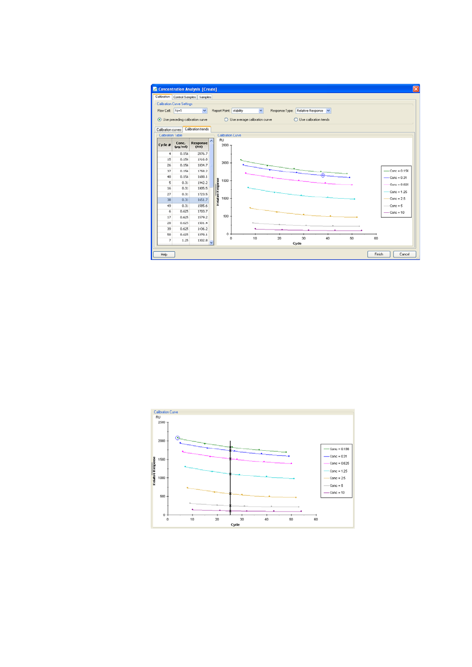
Biacore T200 Software Handbook 28-9768-78 Edition AA 145
Concentration analysis 8
If calibration curves are run in replicate (i.e. using the same concentration in two
successive calibration curves with no intervening cycles of another type), the
trends are fitted to points representing the average of replicate measurements.
Right-click on points in the plot or rows in the table for options relating to the
specific calibration sample.
Using calibration trends
Check Use calibration trends on the Calibration tab to create an individual
calibration curve for each cycle in the assay by using interpolated calibration
points from the calibration trend plot. The illustration below shows how the
calibration curve is constructed for cycle 25.
When calibration trends are used, the Calibration tab shows an overlay plot of
the measured calibration curves. Note however that none of these measured
curves is used directly for calibration: an individual (virtual) calibration curve is
constructed for every cycle including the calibration cycles themselves.
The trend lines are extrapolated to cover the cycles in the first and last
calibration cycles so that every cycle has a complete virtual curve. However, if

8 Concentration analysis
8.2 Evaluating calibrated concentration analyses
146 Biacore T200 Software Handbook 28-9768-78 Edition AA
you exclude calibration points at the ends of the trend lines, the trend lines will
not be extrapolated and calibration curves in the regions outside the excluded
range may be incomplete (see illustration below).
Note: When Use calibration trends is selected, results are recalculated
whenever points are excluded from or included in the trend lines, which
can take some time for large runs. For best performance, establish the
trend lines before choosing Use calibration trends.
8.2.3 Control samples
The Control Samples tab displays the measured concentration for control
samples as a plot of response against cycle number.
Numerical results are presented in the table at the left, and plotted as calculated
concentration against cycle number on the right. Select a row in the table to
highlight the corresponding point on the plot.

Biacore T200 Software Handbook 28-9768-78 Edition AA 147
Concentration analysis 8
The table lists the expected concentration as entered for the control samples,
the response and calculated concentration, the calculated concentration as a
percentage of expected and the calibration curve used to calculate the
concentration. Replicate control samples are summarized with average values
and coefficient of variation (CV%) for the response and calculated
concentration.
Right-click on a sample row in the table or a sample point in the plot and choose
Exclude Cycle to exclude that sample from the sample evaluation. Excluded
cycles are shown as open symbols and are marked in the table with red
strikethrough text.
8.2.4 Samples
The Samples tab displays the measured concentrations for samples.
The left-hand panel lists the results sorted by sample ID, with averages and CV
values for each sample ID. The column Calc.Conc. gives the concentration
calculated for the original sample, obtained as the measured concentration
multiplied by the dilution factor. Concentrations for samples that give a
response outside the range of the calibration curve are listed as below or above
the limits of the calibration.
Note: The limits of calibration are defined by the concentrations corresponding
to the response values on the fitted curve for the highest and lowest
calibration samples. Depending on how well the curve fits the
experimental points, these limits may not coincide exactly with the actual
concentrations in the highest and lowest samples.

8 Concentration analysis
8.2 Evaluating calibrated concentration analyses
148 Biacore T200 Software Handbook 28-9768-78 Edition AA
The right-hand panel shows the calibration curve for the currently selected
sample. All sample points calculated from the curve are shown in black:
calibration points are shown in orange. Select a row in the table to highlight the
corresponding point on the plot and vice versa.
Note: If Use calibration trends is selected in the Calibration tab, each sample is
calculated from its own individual calibration curve, shown in the right-
hand panel with a single sample point.
Right-click on a sample row in the table or a sample point on the curve and
choose Exclude Cycle to exclude that sample from the average sample
calculation. Excluded cycles are shown as open symbols and are marked in the
table with red strikethrough text.
8.2.5 Custom models for calibration curves
You can define your own fitting models for calibration curves in concentration
analysis, for example to support validated assay procedures that do not use
linear or 4-parameter calibration fitting. Choose Tools:Models:Concentration
to define or edit fitting models. Models for calibration curves are defined using
similar principles as equation models for kinetics and affinity (see Section 9.9.3).

Biacore T200 Software Handbook 28-9768-78 Edition AA 149
Concentration analysis 8
8.2.6
Evaluating combined result sets
If you use the Append File function to combine result sets from separate runs,
concentration analysis can be evaluated provided that the conditions specified
in Section 5.10 are fulfilled in the combined set. The software does not check the
validity of any evaluation applied to a combined result set, so that it is your
responsibility to determine that the evaluation results are meaningful. It is for
example in principle possible to append a kinetic analysis result file to a
concentration analysis, and then apply concentration analysis evaluation.
Provided that the report point used for the calibration curve also exists in the
cycles from the kinetic run, calculated concentrations will be reported for these
samples.
In order to ensure that concentration analysis is correctly evaluated in
combined result sets, make sure that all files that contribute to the combined
result set are derived from concentration analysis runs. Provided that each file
starts with a calibration curve that is not excluded from the evaluation, the
results will be calculated within the respective files even in the combined result
set. However, if calibration curves at the beginning of files are missing or
excluded, there will be overlap between the individual file sets and some
samples from one file will be evaluated on the basis of calibration curves from
another file. In such cases, it is important to ensure that the calibration curves
and sample analyses in the different files refer to the same analyte and are
performed under as far as possible identical condition.
Note: Beware of using calibration trends with appended result files. If the
appended files use the same calibration concentrations, trends will be
fitted over the whole data set and will be valid only if the response levels
from the different files form a continuous function. The trends will differ
according to the order in which the result files are appended.

8 Concentration analysis
8.3 Evaluating calibration-free measurements
150 Biacore T200 Software Handbook 28-9768-78 Edition AA
8.3 Evaluating calibration-free measurements
Calibration-free concentration analysis calculates the analyte concentration
from the measured mass transport properties and values for the diffusion
coefficient and molecular weight, provided as evaluation variables when the
assay is run (Section B.2). The evaluation is based on fitting the sensorgram data
to a model of 1:1 interaction kinetics, with mass transport parameters
calculated from the supplied diffusion coefficient and molecular weight, and
with the analyte concentration set as a globally fitted variable.
To evaluate calibration-free concentration analysis, choose Concentration
Analysis:Calibration-free from the evaluation toolbar, or choose Add
Concentration Analysis:Calibration-free from the Evaluation menu.
8.3.1 Selecting samples
Choose the samples you want to evaluate in the first dialog:
Sample and cycle list
The table in the top panel lists the samples available for analysis. By default, the
table shows a full list of cycles including details of the flow rate and subtracted
blank cycle (see below) for each sample cycle. Remove the checkmark from
Expand all cycles to collapse the cycle details and show only samples in the
table.

Biacore T200 Software Handbook 28-9768-78 Edition AA 151
Concentration analysis 8
Notes: Selecting a row in the cycle list does not display the corresponding cycle
in the sensorgram panel. Use the selector bar in the sensorgram panel to
view different samples.
The value shown for the diffusion coefficient D is adjusted to the analysis
temperature, and may not be the same as the value for 20°C as entered
when the assay was run.
The option Use reference subtracted data is checked by default if a reference
surface is included in the run setup. You should generally perform the evaluation
using reference-subtracted data, but you can uncheck this option to use
unsubtracted data if you wish.
Remove the check-mark from the Include column to exclude a sample from the
evaluation, or from the Cycle# column in the expanded list to exclude individual
cycles. Remember that each sample must be represented by at least two cycles
with different flow rates for the evaluation to be possible. The initial binding rate
should be clearly higher at the higher flow rate, and should be reliably
measurable (in practice above about 0.2–0.3 RU/s) at the lower flow rate.
It is important that the sensorgrams at the lowest and highest flow rates
(recommended 5 and 100 µl/min respectively) are sufficiently separated. If the
curves are close together or coincide, this indicates that there is not sufficient
mass transport limitation in the binding for reliable concentration
measurement. The table column QC ratio prel provides a guidance value for
this assessment: sufficient mass transport limitation is indicated by a value for
the QC ratio of about 0.2 or higher. You may exclude samples with low QC ratios
before continuing with the evaluation, or include such samples in the data
processing and judge the final results for acceptability.

8 Concentration analysis
8.3 Evaluating calibration-free measurements
152 Biacore T200 Software Handbook 28-9768-78 Edition AA
The QC ratio is calculated as follows from the quotient Q which reflects the
degree of mass transport limitation:
Under conditions of complete mass transport limitation, the binding rate is
proportional to the cube root of the flow rate, so the quotient Q has a value of 1.
When there is no mass transport limitation, the binding rate is independent of
the flow rate so Q has a value equal to the cube root of the flow rate ratio. The
range of possible theoretical values for Q will thus depend on the flow rates used
(for flow rates of 5 and 100 µl/min, the value is 0.37). The QC ratio is calculated
from the measured value for Q normalized to a scale of 0–1:
The Initial rate and QC ratio reported in the Select Samples step are
preliminary values based on the sensorgram data from 7.5 to 12.5 seconds after
the start of the injection. This value may be misleading if the sensorgams are
disturbed. If data is removed from this region (see below) so that initial rates
cannot be calculated, the QC ratio prel is listed as nd (not determined). A final
value, determined from the fitted curves rather than the experimental data, is
presented when the evaluation is complete.
Occasionally, the measured binding rate may be lower at the higher flow rate,
leading to a negative value for the QC ratio. This can occur if the sensorgrams
are disturbed or as a result of experimental variation when the binding rate is
not affected by flow rate (so the binding rates should in theory be equal and the
QC ratio should be 0).
Sensorgram display
The lower panel shows the set of sensorgrams for a selected sample. Select the
sample to display with the selector bar. By default, this panel shows data after
subtraction of blank cycles (see below). Uncheck Show blank subtracted data
to see the unsubtracted data and the corresponding blank sensorgrams (shown
in gray).
Note: The evaluation will always use blank-subtracted data where possible,
even if this first dialog shows unsubtracted data.
quotient Q
initial rate at high flow rate
initial rate at low flow rate
-------------------------------------------------------------------
low flow rate
high flow rate
----------------------------------
3
×=
Q
max
1=
Q
min
low flow rate
high flow rate
----------------------------------
3
=
QC ratio
Q
measured
Q
min
–
Q
max
Q
min
–
-----------------------------------------
=

Biacore T200 Software Handbook 28-9768-78 Edition AA 153
Concentration analysis 8
With the option Show original sensorgrams checked, the sensorgram panel
shows the full sensorgrams for the sample injection. Uncheck this option to
show the data that will be used in the fitting. The range of data used is indicated
by blue vertical lines, and any data removed from the sensorgrams is not shown.
Blank subtraction
Blank cycles are identified by the value y or yes in the Blank keyword (Section
B.2), and must have the same flow rate and injection time as the sample cycles
from which they are subtracted. If there is no preceding blank cycle, the nearest
following one is used. If there is no blank cycle available for one or more of the
cycles in a sample series, the evaluation will be performed using data without
blank subtraction for that series.
Click Included blanks to display an overlay plot of blank cycles in the run.

8 Concentration analysis
8.3 Evaluating calibration-free measurements
154 Biacore T200 Software Handbook 28-9768-78 Edition AA
Remove the check-mark from the Include column to exclude a blank cycle from
the evaluation (for example if the sensorgram shows unreasonable response
levels or unacceptable disturbances).
Setting fitting ranges and removing disturbed data
Click Advanced settings if you want to adjust the range of data that will be used
in the evaluation and/or remove disturbances from the data.
Choose whether you want to make the changes on all sample series in one
operation or on selected single sample series. You cannot separate the
individual sensorgrams in a sample series.
To adjust the fitting range, drag the blue vertical lines that mark the limits of the
range. The default range is from 10 seconds before the start of the injection to
5 seconds before the end. Including baseline data before the start of the
injection helps to ensure robust evaluation of the data.

Biacore T200 Software Handbook 28-9768-78 Edition AA 155
Concentration analysis 8
Note: If you adjust the fitting range differently for different sample series, the
range indicators will not be shown when you display All sample series.
Evaluation items with different ranges for different sample series cannot
be saved in evaluation methods (Section 6.8).
To remove disturbed data, drag with the right mouse button to select the data,
then click Remove Selection. Click Undo to restore deleted data.
8.3.2 Performing the evaluation
When you are satisfied with the data selection, click Next to start the evaluation.
Results appear in the table as each sample series is completed. The evaluation
progress is shown in the sensorgram panel.
The fitting procedure is normally fast. If fitting appears to hang for a particular
sample series, you can click Accept to accept the current fitting results for that
series or Abort current to abandon the series. Click Abort remaining if you want
to abandon all remaining series in the evaluation. The fit status is recorded in the
table of results.
Click Expand all cycles in the finished result display to display the details of the
sample series in the cycle list.
The results are reported in terms of Measured Conc, which is the value
calculated from the fitting, and Calc Conc which is obtained by multiplying the
Measured Conc by the dilution factor to give the concentration in the original
sample. You can change the units for the reported concentration in the header
for the Measured Conc column.

8 Concentration analysis
8.3 Evaluating calibration-free measurements
156 Biacore T200 Software Handbook 28-9768-78 Edition AA
Notes: The diffusion coefficient D listed in the evaluation results is the value at
the analysis temperature, calculated automatically in the software from
the value at 20°C provided when the assay is run.
The Initial rate and QC ratio in the finished evaluation are calculated from
the fitted curves and are therefore not affected by sensorgram
disturbances or data removal.
If the fitting fails
If the sensorgrams appear to be satisfactory on visual inspection and quality
assessment but the evaluation fails to fit the experimental data, it may help to
adjust the initial values for fitting parameters. To do this, step back to the Select
samples dialog, open the Advanced settings and click Parameters. Try in the
first place changing the starting value for Conc by several orders of magnitude,
either up or down. A typical example of a failed fitting is shown below (this was
obtained using an initial value for Conc of 1e-3 where a value of 1e-6 is more
appropriate).
8.3.3 Interpreting the results
Consider the following aspects of calibration-free concentration analysis when
interpreting the results:
• Check the appearance of the sensorgrams and fitted curves. Reject
samples where the fit is poor at one or both of the flow rates. Use the Chi2
(chi-squared) value as a guideline for fitting quality: this value should be
low in relation to the maximum measured response. As a rough guideline,
acceptable chi-squared values should be less than about 5% of the
response reached at the end of the sample injection at the lowest flow rate
(disregarding the difference in units between chi-squared and response).
•Check the QC ratio. Treat the results with caution if the value is lower than
about 0.2.

Biacore T200 Software Handbook 28-9768-78 Edition AA 157
Concentration analysis 8
• Check the value for SE (Conc) or T (Conc). This value represents the
statistical significance of the calculated concentration, and is shown as
standard error (SE) or T-value (see Section 9.4.2) according to the setting in
Tools:Preferences. Reject samples where the standard error is more than
about 20% of the calculated concentration (or correspondingly the T-value
is lower than about 5).
• The optimal concentration range that can be measured with calibration-
free concentration analysis is 0.5-50 nM. Values for Meas. Conc outside
this range should be treated with caution.
8.3.4 Fitting model
Evaluation of calibration-free concentration relies on fitting the data to a model
for 1:1 interaction (see Section 9.8.1) where the mass transport coefficient is
provided (through calculation from the diffusion coefficient, and flow cell
characteristics) and the analyte concentration is evaluated as a global variable.
Although this model is equivalent to the model for evaluation of 1:1 kinetics in
terms of the interaction description, the model for calibration-free
concentration analysis cannot be accessed through the model editor.
Notes: The diffusion coefficient for the analyte at the analysis temperature is
calculated automatically from the value at 20°C. The value at 20°C is
provided as an evaluation variable when the assay is run (Section B.2).
Parameters for calculating the mass transport coefficient from the
diffusion coefficient are fixed in the software.

8 Concentration analysis
8.3 Evaluating calibration-free measurements
158 Biacore T200 Software Handbook 28-9768-78 Edition AA

Biacore T200 Software Handbook 28-9768-78 Edition AA 159
Kinetics and affinity analysis 9
9 Kinetics and affinity analysis
Biacore T200 offers three main functions for analysis of interaction kinetics and
affinity:
• Kinetics and affinity measurements on the sensor surface, which
determine the interaction characteristics between ligand and analyte.
Kinetic parameters are evaluated from the association and dissociation
phases of the sensorgram, and affinity either from the kinetic parameters
or from plots of steady-state analyte binding levels (R
eq
) against
concentration.
• Thermodynamic analysis, which relies on measurement of either kinetics
or affinity at different temperatures.
• Affinity in solution, where the interactants are mixed in known
concentrations in solution and allowed to reach equilibrium. Biacore T200
is then used to determine the concentration of free interactant in
equilibrium with the complex.
Kinetic constants derived from surface interaction measurements in multiple
separate experiments can be collated and summarized in the separate
Biacore T200 Kinetic Summary software (Section 9.6).
This chapter describes how to evaluate surface-bound kinetics and affinity. If
there are multiple sample series in the same data set, evaluation can be
performed either in single mode (where each sample series is evaluated
separately with interactive control over several aspects of the evaluation), or in
batch mode (where multiple series are evaluated automatically using default
settings).
Thermodynamic analysis and measurement of affinity in solution are described
in Chapters 10 and 11 respectively.
Kinetics and affinity are normally determined from the binding characteristics
of a series of analyte concentrations. These concentrations may be injected in
separate cycles with surface regeneration between the cycles (multi-cycle
analysis) or sequentially in a single cycle with no regeneration between
injections (single-cycle analysis), as illustrated in Figure 9-1. Results from these
two approaches are evaluated in the same way, using the same tools and fitting
models, and may even be evaluated together in a single evaluation. Significant
differences in evaluation appearance between the approaches are illustrated
where relevant in this chapter.
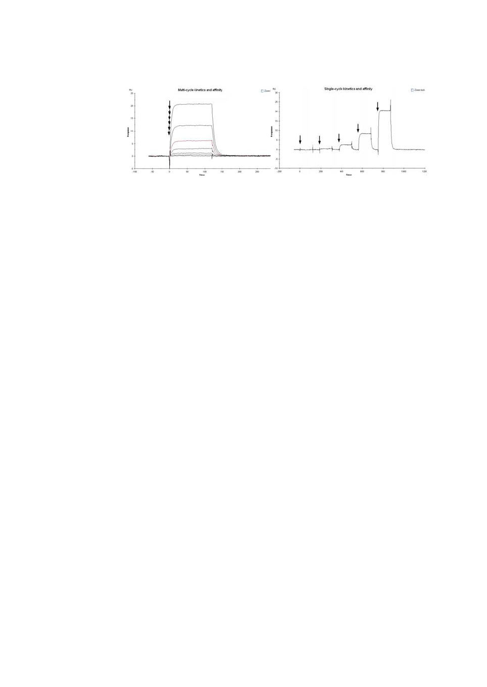
9 Kinetics and affinity analysis
9.1 Requirements for kinetics and affinity evaluation
160 Biacore T200 Software Handbook 28-9768-78 Edition AA
Figure 9-1. In multi-cycle kinetics and affinity determinations, each sample is injected in
a separate cycle. The concentration series is presented as an overlay plot aligned at the
start of the injection in the evaluation software.
In single-cycle determinations, the samples are injected sequentially in the same cycle.
Arrows in the illustrations mark the start of sample injections.
9.1 Requirements for kinetics and affinity evaluation
The minimum requirements for evaluation of kinetics or affinity are one cycle
with a Sample injection in an assay step with purpose Sample, and with the
sample concentration in the keyword Conc. If the concentration is not given in
molar-based units, the keyword MW must also be included with a value for the
molecular weight. For method-based runs, the method must be correctly
constructed as described in Section 5.10.2: if necessary, the keyword table can
be edited so that the conditions are met in full (see Section 6.6). Note however
that the command type cannot be edited in the keyword table. Refer to
Chapter 5 for details of how to construct methods in Method Builder.
The recommended minimum conditions for kinetic and affinity evaluation are:
• a concentration series of analyte with at least four non-zero
concentrations
• at least one blank cycle consisting of zero concentration sample (for
single-cycle kinetics the blank cycle must replicate the sequence of
injections in the analysis cycle)
• for multi-cycle kinetics, duplicate determinations for at least one non-zero
concentration.
These conditions are recommended but not mandatory in the Kinetics/Affinity
wizard.

Biacore T200 Software Handbook 28-9768-78 Edition AA 161
Kinetics and affinity analysis 9
9.2 Evaluating kinetics and affinity in single mode
9.2.1 Basic procedure
To start a kinetics or affinity evaluation in single mode, choose Surface-bound
kinetics/Affinity from the Kinetics/Affinity button on the toolbar or the Add
Kinetics/Affinity in the Evaluation menu. Check the Single mode option in the
first dialog.
1 The first dialog presents the concentration series available in the current
result set and allows you to choose the curves included in the evaluation.
A concentration series is defined by a set of curves with the same sample
name, analysis temperature and curve identity. Select the concentration
series you want to work with in the respective pull-down lists.
Note: For runs with immobilized ligand, there will be only one choice for
Ligand name. Multiple choices may be available if the ligand is
captured and varies between cycles.
For single-cycle kinetics, the cycles table lists all concentrations injected in each
cycle. You can however only include or exclude whole cycles at this stage.

9 Kinetics and affinity analysis
9.2 Evaluating kinetics and affinity in single mode
162 Biacore T200 Software Handbook 28-9768-78 Edition AA
Note: Sample names are case-sensitive, so that “Sample” and “sample”
belong to different concentration series. Edit the sample names in the
keyword table if you have unintentionally mixed upper- and lower-
case letters.
If the result set contains data from more than one file, curves with the same
ligand, sample name, temperature and curve identity are grouped together
in a single concentration series.
Use the Include column in the table of curves to choose which curves
should be included in the data set to be evaluated. You can select several
curves and use the right-click menu to exclude or include multiple curves in
one operation. By default, all curves for the sample are included.
Sensorgrams for non-zero concentrations are shown in color, and those for
blanks (zero concentrations) in light gray. The sensorgrams are adjusted to
zero at the start of the sample injection on both the response and time axes.
The average of the blank sensorgrams will be automatically subtracted
from the other curves when you proceed to the next step. If you do not want
to perform blank subtraction, exclude the zero concentration sensorgrams
from the data set. You can also choose to use blanks from other
concentration series for blank subtraction: these are listed at the bottom of
the table, and are excluded by default. Only blank sensorgrams with the
same contact and dissociation times as the samples are used.
The three check-boxes below the sensorgram panel control the type of
curves shown in the display. You can use these check-boxes to examine the
sample and blank curves without interference from each other, and to
show the average blank that will be used for subtraction. Bear in mind
however that these boxes control the display only and do not affect the
data set that will be evaluated.
If you have multiple ligand densities represented in the result set, click
Multiple Rmax to assign curves to the different sets (see Section 9.2.2).
Click Adjust Injection Events if you want to adjust the injection start and
end positions for the evaluation. These positions are set automatically from
the event markers in the run, but may need slight adjustment for best fitting
to fast interaction processes. The adjustment compensates for small
systematic discrepancies in the interval between the event as recorded in

Biacore T200 Software Handbook 28-9768-78 Edition AA 163
Kinetics and affinity analysis 9
the event log and the time that the sample actually reaches the detection
spot on the sensor surface. The difference is most apparent at low flow
rates.
The event markers for injection start and end in the result file are shown on
the x-axis. Drag the vertical reference lines to adjust the injection start or
end point for evaluation. You can adjust the events by ±10 s from the
original position. The same adjustment is applied to all curves in the data
set, whether they are currently included for evaluation or not. This function
cannot be used for single-cycle kinetics, for evaluations with mixed single-
and multi-cycle analyses, or for multi-cycle analyses with different contact
times in different cycles.
Note: If you adjust the injection start, the time axis in the evaluated data is
adjusted correspondingly so that the start of the injection is always
at time zero. The display in the Adjust injection events dialog
however always shows the original time axis, with zero at the event
marker in the run data.

9 Kinetics and affinity analysis
9.2 Evaluating kinetics and affinity in single mode
164 Biacore T200 Software Handbook 28-9768-78 Edition AA
2 The second dialog shows the blank subtracted curve set and allows you to
delete selected regions from all or selected curves, for example to eliminate
spikes or other disturbances.
To delete a selected region from all curves, drag with the right mouse
button over the region to be deleted and click Remove Selection. Click
Undo to restore the deleted data.
If you want to delete a region from only selected curves, remove the
checkmark from the Edit column in the table for the curves that are to be
left unchanged. All curves are selected by default and are shown in dark
color. Curves that are not selected for editing are shown in light color. Note
that all curves will be evaluated, whether they are selected for editing or
not: removing the Edit checkmark does not exclude a curve from the data
set for evaluation.
Note: For best resolution of fast kinetics, you should delete any
disturbances in connection with injection start and stop (see
illustration below). These are commonly caused by small
misalignments in reference and blank subtraction, leading to spikes
at the beginning and end of the injection. The effect of subtraction
spikes on the calculated kinetic constants is usually negligible except
for very fast interactions.

Biacore T200 Software Handbook 28-9768-78 Edition AA 165
Kinetics and affinity analysis 9
Click Affinity for steady state affinity evaluation or Kinetics for kinetics
evaluation when you are satisfied with the curves.
3(Affinity only). If you choose to evaluate steady state affinity, the next
dialog gives a preview of the plot of steady state response against
concentration, with the option to adjust the selection of data used to
calculate response values.
The top panel shows the plot of R
eq
against C, based on average response
values over the region marked on the sensorgrams. Click Settings to adjust
the region used for calculation of R
eq
values.

9 Kinetics and affinity analysis
9.2 Evaluating kinetics and affinity in single mode
166 Biacore T200 Software Handbook 28-9768-78 Edition AA
For single-cycle affinity runs, the same settings are applied to each
injection in the cycle.
Click Next> when you are satisfied with the data selection.
4 In the next dialog (applicable to both Kinetics and Affinity), you select the
fitting model and perform the fit. The same data can be fitted repeatedly
to different models or to the same model with different settings.
Select the model from the pull-down list. Available models are described in
Section 9.8. Click Parameters if you want to change the starting values or
scope of any of the parameters (see Section 9.7.2 for details), then click Fit
to perform the fitting.
During the fitting procedure, the fitted curves are shown in black overlaid
on the experimental data. Fitting progress is indicated in the sensorgram
window by display of the iteration number, the current chi-squared value
and the relative change in the parameter that was changed most from the
previous iteration. You can use the Abort or Accept buttons to cancel the
fitting or accept the fitting after the current iteration. You may want to
cancel the fitting if it is clear that a fit cannot be found, or to accept the
fitting if the chi-squared value and/or maximum relative change indicate
that an acceptable fit has been achieved. Clicking on Accept will stop the
fitting at the end of the current iteration, which may take a few moments to

Biacore T200 Software Handbook 28-9768-78 Edition AA 167
Kinetics and affinity analysis 9
complete.
You can enter a short description for the fit in the Description box. This can
be useful for example to distinguish different fits for thermodynamic
analysis (Section 10.2).
To perform additional fits on the same data, choose a new model or new
parameter settings and click Fit. To remove a fit from the evaluation item,
select the fit in the list of current fits and click Delete.
Click Finish to complete the evaluation and place the item in the evaluation
explorer panel. You can click Back to review the choice of data for the
evaluation: however, if you make any changes to the data (e.g. remove
additional sections from a curve or exclude a curve from the set), all current
fits will be deleted. Current fits are also deleted if you switch between
kinetics and affinity evaluation.
Kinetics results
When the fit is completed, the results for kinetics are displayed as fitted curves
overlaid in black on the experimental data, with details in the table below the
curves:
The detailed results are presented on four tabs:
• Quality control summarizes important aspects of the quality of the fitting,
as an aid to judging the reliability of the reported results. The quality
control criteria are discussed in Section 9.4.1. This tab is only shown for
kinetic evaluations using the predefined 1:1 model.

9 Kinetics and affinity analysis
9.2 Evaluating kinetics and affinity in single mode
168 Biacore T200 Software Handbook 28-9768-78 Edition AA
• Report shows selected parameters and calculated values. The contents of
the Report tab are defined in the model. Global parameters are listed on a
single row at the top of the table, and local parameters are listed on one
row for each curve.
• Residuals plots the difference between the experimental and fitted curves
for each point in the curves. Use this display as an aid in judging how
closely the results fit the experimental data.
• Parameters shows the values for all parameters in the fitting equations.
Affinity results
For affinity determination, the reported K
D
value is marked on the plot as a
vertical line (for a 1:1 interaction, K
D
is the same as the analyte concentration at
a response equal to half R
max
). If the reported value is higher than half the
highest concentration used, this line will be shown broken in red as a warning
that the value may be unreliable because the plot does not flatten out
sufficiently.
The detailed results are presented on two tabs:
• Report shows selected parameters and calculated values. The contents of
the Report tab are defined in the model. Global parameters are listed on a
single row at the top of the table, and local parameters are listed on one
row for each curve.
• Parameters shows the values for all parameters in the fitting equations.

Biacore T200 Software Handbook 28-9768-78 Edition AA 169
Kinetics and affinity analysis 9
9.2.2 Multiple ligand densities
Analysis of the same analyte concentration series over multiple ligand densities
can provide more robust fitting than a single ligand density. The kinetic and
steady-state affinity fitting functions support simultaneous analysis of up to five
sets of data with independent values for R
max
, returning a single set of rate
constants for the whole combined data set. Analyses over multiple ligand
densities may be performed in separate runs that are combined with the
Append file function, but should preferably be performed on multiple flow cells
in the same run to ensure that the experimental conditions are comparable as
far as possible.
To set up evaluation of the same sample series over multiple ligand densities,
click Multiple Rmax in the first dialog box for kinetics and affinity evaluation. A
panel for data subsets representing different R
max
values opens to the left of the
curve table.
Click Add to add a new data subset. If you have multiple sets of the currently
chosen curve type in the evaluation session (e.g. multiple reference subtracted
curves), the next curve in the list is assigned to the new data subset. If there are
no more curves of the same type available, the new set will be a copy of the
most recently created subset. You can add up to five data subsets, representing
five ligand densities. The same sample name and analysis temperature apply to
all subsets.
Click on a subset to manage the contents of the subset. You cannot mix subsets
that use different samples or different temperatures.

9 Kinetics and affinity analysis
9.3 Batch mode evaluation
170 Biacore T200 Software Handbook 28-9768-78 Edition AA
The subsets will be evaluated together, with rate or affinity constants that are
global for the whole data set and R
max
values that are global within each subset
but can differ between subsets.
Note: The Parameters tab in evaluation of kinetics with a global R
max
parameter within subsets lists a parameter i
n
which is set to 1 for the n
th
subset and 0 for all others. This is used to control R
max
values for each
subset: values are fitted as Rmax
×
i
n
, which returns a non-zero value for
the n
th
subset only. For affinity evaluations, each subset is represented by
one curve and R
max
is simply evaluated as a local parameter.
9.3 Batch mode evaluation
Batch mode allows you to evaluate multiple sample series (e.g. different
analytes interacting with a common ligand, or measurement of the same
interaction at different temperatures) automatically. You select the series to be
evaluated and the fitting model to be used, and evaluation is carried to
completion without further intervention.
To perform evaluation in batch mode, start the kinetics/affinity evaluation
(Section 9.2.1) and check the Batch mode option in the first dialog.
IMPORTANT! Make sure that the same curve numbers are not assigned to
more than one data subset. If a curve is assigned to two data sets, the
software will try to evaluate the same curve with two different Rmax values,
and the fitting may be distorted.
Do not evaluate multiple copies of the same subset for multiple ligand
densities. Subsets that are duplicated will be weighted more than those that
are not duplicated in the fitting procedure.
Do not attempt to use subsets for any purpose other than multiple ligand
densities. The data will be evaluated in terms of multiple ligand densities
regardless of how you have assigned curves to the subsets.

Biacore T200 Software Handbook 28-9768-78 Edition AA 171
Kinetics and affinity analysis 9
Choose the Evaluation purpose as kinetics or affinity, and choose the fitting
model. Click the Parameters button if you want to make adjustments to the
fitting parameters (see Section 9.2.1). The same model and parameter settings
will be used for all evaluations in the batch.
Choose the curve type to use (you should normally evaluate reference-
subtracted curves) and check the data sets you want to evaluate in the table.
Click Finish to perform the evaluation. One evaluation item will be created for
each sample series.
Notes: A data set for batch evaluation is defined as a set of cycles with the same
ligand, sample and analysis temperature. Blank cycles will be subtracted
within each data set.
Evaluation in batch mode does not support multiple ligand densities,
adjustment of injection start, selection of blank cycles or removal of
selected data. Individual evaluation items created during batch
evaluation can however be edited separately.

9 Kinetics and affinity analysis
9.4 Quality assessment for kinetics evaluation
172 Biacore T200 Software Handbook 28-9768-78 Edition AA
9.4 Quality assessment for kinetics evaluation
9.4.1 The Quality Control tab
The Quality Control tab in the kinetic evaluation results (for evaluations using
the predefined 1:1 model only) gives a brief overview of the reliability of the
results. If you prefer, you can hide the quality control tab by setting the
appropriate option in Tools:Preferences on the main menu.
The symbols used on this tab have the following meanings:
The quality of the fitting is assessed in five areas:
Magnitude of kinetic constants
If either association or dissociation rate constants are close to or outside the
limits that can be determined in the instrument, this will be reported. For values
close to the limit, judge the validity of the results on other assessment criteria
as described in this chapter.
Parameter uniqueness
In some situations, it may be possible to determine a value for a combined
function of two or more parameters without being able to determine unique
values for the individual parameters. Such parameters are said to be correlated.
One example is the pair of kinetic rate constants k
a
and k
d
, that are related
through the affinity constant K
D
(K
D
= k
d
/k
a
): it may be possible to determine the
affinity constant reliably without being able to resolve the individual rate
constants.
(Green) Pass: quality assessment acceptable.
(Yellow) Warning: quality assessment close to the limits of
acceptability
(Red) Fail: quality assessment unacceptable
(Blue) User assessment recommendations

Biacore T200 Software Handbook 28-9768-78 Edition AA 173
Kinetics and affinity analysis 9
Parameter uniqueness is assessed by testing correlation between pairs of the
parameters k
a
, k
d
and R
max
. If significant correlation is found, this will be
reported as a warning that parameters cannot be uniquely determined.
Note: This test does not explore all possible parameter correlations. A Pass
status for this test is not a fail-safe indication that parameters are
uniquely determined.
The Check Kinetic Data tool (Section 9.4.4) provides a visualization of potential
correlation between k
a
and k
d
.
Bulk refractive index
After reference subtraction and blank subtraction, sensorgrams for kinetic
evaluation should not in principle contain any bulk refractive index shifts
(parameter RI in predefined models). However, there may be some
circumstances where small bulk refractive index shifts may remain in reference-
and blank-subtracted data. On the other hand, the fitting algorithm tends to
interpret rapid interaction events (incorrectly) as bulk shifts. If the fitting returns
significant values for RI, a warning will be issued in the quality control tab.
Examine the sensorgrams and fitted curves to determine whether bulk shifts as
reported by the fitting are true or false. In cases where reported bulk shifts are
unreasonably large, you may want to set RI to a constant value of zero in the
Parameters setting for the fitting. If you do this, the bulk contributions
component in the quality control tab will be reported as neutral since the RI
parameter was not evaluated.
Sensorgram curvature
You should check that the sensorgrams have sufficient curvature for kinetic
determination. Ideally, the sensorgrams for at least the one or two highest
concentrations should show measurable binding rates at the beginning of the
sample injection and approach a steady state towards the end of the injection.
Sensorgrams that approximate to “square-wave” pulses (indicating rapid
association and dissociation) and those that do not flatten out during the
injection generally do not contain sufficient kinetic information for reliable
evaluation. Ideally, the dissociation phase should be long enough to monitor a
fall in response of at least 10-15% of the starting value.

9 Kinetics and affinity analysis
9.4 Quality assessment for kinetics evaluation
174 Biacore T200 Software Handbook 28-9768-78 Edition AA
Figure 9-2. Examples of sufficient and insufficient sensorgram curvature.
Top: Ideal sensorgrams approaching steady state during sample injection and returning
to baseline during dissociation.
Bottom left: Rapid interaction approaching “square wave” appearance. These
sensorgrams return rate constants close to the limit of measurement for the instrument.
Bottom right: Slow association and dissociation, giving insufficient curvature in both
association and dissociation phases. Evaluation is possible but will not be very reliable.
If the interaction is too fast to provide kinetic information, you may only be able
to determine affinity constants. Interactions that do flatten out sufficiently
during the injection or dissociate sufficiently during the dissociation phase may
sometimes be analyzed by prolonging the association or dissociation phase
respectively.
Residuals
You should check that the residuals (the difference between experimental and
fitted value for each data point in the sensorgrams) lie within reasonable limits.
For a perfect fit, the residuals reflect the short-term noise in the sensorgrams
and scatter around zero (typically ±1-2 RU). Systematic deviations, seen as a
definite shape in the residual plot, indicate that the interaction model is to a
greater or lesser extent unsuitable for the interaction. As an aid in judging the
residuals, guidelines are drawn on the residual plot to indicate the range of
acceptability. Most of the residuals should be within the inner (green) limits.
Figure 9-3. The residuals for a good fit (left) scatter around 0, ideally in a random
distribution representing the noise in the sensorgrams. For a poor fit (right) the residual
curves show a definite shape and deviate farther from 0.

Biacore T200 Software Handbook 28-9768-78 Edition AA 175
Kinetics and affinity analysis 9
The guideline positions are calculated in relation to the response range of the
sensorgrams. The guidelines are only shown for evaluations using the
predefined 1:1 model (i.e. when the quality control tab is included).
9.4.2 Statistical parameters
Two statistical parameters are provided to help in assessing the results:
• Chi-squared is an indicator of how closely the fitted curves agree with the
experimental data. One chi-squared value is reported for the whole fitting.
• Standard error or T-value is an indicator of parameter significance, and is
reported separately for each fitted parameter.
Chi-squared
Chi-squared is a measure of the average squared residual (the difference
between the experimental data and the fitted curve), calculated as:
For sensorgram data, the number of data points is very much larger than the
number of fitted parameters in the model, so
and chi-squared reduces to the average squared residual per data point. If the
model fits the experimental data precisely, chi-squared represents the mean
square of the signal noise.
IMPORTANT! Use the Quality Control assessment as a help in making your
own judgement of the results. Pass status in the quality control parameters
does not necessarily indicate that the fit is acceptable or that the results are
biologically relevant. On the other hand, Fail status in any of the parameters
is a reliable warning indicator.
Base your assessment on the overall quality of the results and the fitting,
taking all quality control parameters into account.
where r
f
is the fitted value at a given point
r
x
is the experimental value at the same point
n is the number of data points
p is the number of fitted parameters
chi-squared
r
f
r
x
–()
2
1
n
∑
np–
----------------------------
=
npn≈–

9 Kinetics and affinity analysis
9.4 Quality assessment for kinetics evaluation
176 Biacore T200 Software Handbook 28-9768-78 Edition AA
Chi-squared is listed on the Report tab.
Standard error and T-value
The significance of parameter values is indicated by the standard error (SE) or T-
value listed on the Parameters tab in the fitting results. This is a statistical
indication of the significance of a fitted parameter. Lower standard error values
indicate higher significance: if the standard error represents less than 10% of
the parameter value, the parameter is significant for the experimental data.
For ease of comparison between parameters with widely different absolute
values (e.g. k
a
and k
d
), the standard error may be expressed as a T-value, which
is obtained by dividing the value of the parameter by the standard error. A high
T-value corresponds to a low standard error. As a general guideline, parameters
with a T-value greater than about 10 should be regarded as significant.
The choice of whether to display parameter significance as standard error or T-
value is made on the Fit tab of the Tools:Preferences dialog.
The significance of a parameter is a measure of how much a change in the
parameter value affects the closeness of fit. A parameter with low significance
can have a wide range of values without affecting the fit. Typically (but not
always), parameters with a low significance have unreasonable values: for
example typical values for the mass transfer constant for proteins are around
10
8
RU·M
-1
s
-1
, but evaluation of data with no mass transfer limitation might
return a value of 10
12
or higher. Similarly, rate constants that lack significance
are often assigned values outside the reasonable range for biomolecular
interactions, or outside the range that can be measured with Biacore.
Notes: The standard error and the Check Kinetic Data tool assess parameter
significance in different ways, even if the results of the assessment may
sometimes be related. Check Kinetic Data tests the contribution of a
group of parameters (rate constants for the interaction and mass
transport processes) to the closeness of fit by examining the results of
correlated changes, whereas the standard error is a mathematical
assessment of the significance of a single parameter. If the Check Kinetic
Data tool indicates that the rate constants are not significant, the
standard error for the constants may be expected to be high. However,
the converse is not always true (a high standard error will not always be
reflected in the behavior of the Check Kinetic Data tool).
Even if parameters with low significance can have a wide range of values
without affecting the fit, repeated evaluation of the same data set will
always return the same value for all parameters. Consistency of a value
between repeated evaluations is not a test of significance.

Biacore T200 Software Handbook 28-9768-78 Edition AA 177
Kinetics and affinity analysis 9
U-value
The U-value is an estimate of the uniqueness of the calculated values for rate
constants and R
max. If parameters are correlated (see Section 9.4.1), the fitting
procedure can determine their relative magnitudes but not absolute values (for
example, knowing the affinity gives the ratio but not the values for rate
constants). The U-value is determined by testing the dependence of the fit on
correlated variations in pairs of parameters, and is reported on the Report tab
as a single value for the whole fitting. U-values above about 25 indicate that
absolute values for two or more of the parameters (rate constants and R
max) are
correlated and cannot be determined. If the U-value is below about 15 the
parameter values are not significantly correlated.
9.4.3 Components of the fit
Choose Tools:Components from the fitted results window to display a plot
showing the contribution of components in the interaction model to the fitted
curve. Choose which cycle to display in the selector bar.
The example illustrated here is taken from a fitting to a bivalent analyte model
(see Section 9.8.2), and shows clearly how the component AB2 (analyte attached
to the surface through both binding sites) is displaced by AB as the interaction
progresses.
9.4.4 Check kinetic data
Kinetic constants obtained from the fitting procedure are only significant if the
observed binding is not seriously limited by mass transport of analyte to the
surface (see Section 9.8). For 1:1 fitting results, you can check whether mass
transport is limiting or not using the Check Kinetic Data function.

9 Kinetics and affinity analysis
9.4 Quality assessment for kinetics evaluation
178 Biacore T200 Software Handbook 28-9768-78 Edition AA
Choose Tools:Check Kinetic Data to open a dialog that displays simulated
sensorgrams based on the fitting results, with the interaction rate constants k
a
and k
d
varied in parallel (so that the affinity constant, remains unchanged). If
curves do not shift as values for k
a
and k
d
are changed, this means that the
actual values are not important for the fitting, and the curves do not contain
kinetic information. Conversely, if the simulated curve shape changes as the
values of k
a
and k
d
are varied, the fitting is dependent on the actual values and
the curves do contain kinetic information.
This tool is only available for results obtained with the 1:1 fitting model.
(This example illustrates a fitting with only three concentrations for clarity.)
To use the tool, drag the slider for the modification factor M and observe the
behavior of the curve display. The original curves (which remain unchanged as
you drag the slider) are shown in black: blue curves show the simulation for k
a
and k
d
multiplied by M, while red curves show the simulation for k
a
and k
d
divided by M. If the red (reduced rate constants) and blue (increased rate
constants) curves clearly diverge from the original curves, the fitting is sensitive
to changes in the rate constants and the curves probably contain significant

Biacore T200 Software Handbook 28-9768-78 Edition AA 179
Kinetics and affinity analysis 9
kinetic information. If on the other hand the divergence is negligible, the values
of the rate constants do not matter because the binding is fully limited by mass
transfer. Mass transfer places an upper limit on the rate constants that can be
measured: on the borderline, the fitting is sensitive to a reduction in rate
constants but not to an increase.
Choose the Residuals option in the Compare to frame to examine the effect of
varying the modification factor on the difference between the original and
modif ied curves in relation to the experimental residuals. The tool display allows
the simulated difference curves to be compared to the experimental residuals
or to residuals averaged over a moving time window. The latter option smooths
the experimental residual display, making it easier to observe the general shape
of the residual curves. Movable horizontal Limit guides can be displayed to
mark the extent of the residual variation and aid visual interpretation. (Note that
the limit guides are not related to the guidelines shown on the residual tab for
QC purposes (Section 9.4.1), and do not in any way imply acceptance limits.)
Figure 9-4. Kinetic data check comparison to residuals (left) and averaged residuals (right).
9.5 Quality assessment for affinity evaluation
Steady state affinity evaluations are performed by fitting a plot of R
eq
against
concentration C to a model representing equilibrium 1:1 binding. The closeness
of fit is reported as a chi-squared value, calculated in the same way as for
kinetics. Note however that the number of points in the steady state affinity plot
is very much lower than for kinetic evaluation, so that chi-squared is a more
sensitive indicator of fitting quality.
The plot of R
eq
against C approaches a limiting value (equivalent to R
max
) at very
high concentrations. Robust evaluation of the data requires that the plot shows
sufficient curvature for reliable estimation of R
max
. As a rule of thumb, the
evaluation is acceptable only if the calculated K
D
value is less than half the
highest analyte concentration used. (For a 1:1 interaction, the K
D
value is equal
to the analyte concentration that gives 50% saturation of the binding sites, so
that R
eq
=0.5R
max
. In other words, reliable evaluation is only obtained if the
surface is more than 50% saturated at the highest analyte concentration.)

9 Kinetics and affinity analysis
9.6 Summarizing kinetics and affinity results
180 Biacore T200 Software Handbook 28-9768-78 Edition AA
To help in this assessment, the calculated K
D
value is indicated as a vertical line
at the corresponding analyte concentration. The line is red and broken if the
value is greater than half the highest concentration.
Figure 9-5. For reliable evaluation, the calculated K
D
value should be less than half the
highest analyte concentration used. When this condition is met, the K
D
value is indicated
with a full black line in the result plot (left). When the condition is not met, the K
D
value is
indicated with a broken red line.
9.6 Summarizing kinetics and affinity results
You can summarize the kinetics and affinity evaluation results from several runs
or from several evaluation items for the same run using the separate
Biacore T200 Kinetics Summary software (this is installed automatically
together with the Evaluation Software).
9.6.1 Creating kinetic summaries
To create a kinetic summary of the results in a single evaluation file, simply open
the evaluation file (file type .bme) in the Kinetics Summary software. The
Kinetics Summary software can also be started from the Tools menu in the
Evaluation Software.
To create a summary of the results in multiple files, you can either select multiple
files within the same folder in the Open dialog box using Ctrl-click and/or Shift-
click, or use File:Append File to add results to an existing summary. You can
open saved summary files (file type .bks) in addition to evaluation files.
9.6.2 Basic summary presentation
The summarized kinetic and affinity results are presented as thumbnail plots of
the kinetics and evaluation items and as a table of result data. Multiple fits in the
same item in the Evaluation Software are presented as separate fits in the
summary.

Biacore T200 Software Handbook 28-9768-78 Edition AA 181
Kinetics and affinity analysis 9
Thumbnail types
Thumbnails can be displayed as small, standard or extended diagrams, selected
from the View menu or from the options under the Thumbnails button.
Thumbnail display settings
Choose Display Settings from the View menu or the right-click menu for display
settings for the thumbnails.
Small Provides an overview of many thumbnails for general comparison.
Details will not be legible in the thumbnails. Individual thumbnails
are identified in a tool tip.
Standard Shows the thumbnails with identification, legible axis, and a
summary of fitting model and kinetic or affinity constants.
Extended Shows more detailed identification of each thumbnail than the
standard view.

9 Kinetics and affinity analysis
9.6 Summarizing kinetics and affinity results
182 Biacore T200 Software Handbook 28-9768-78 Edition AA
If you choose to use the same x- and/or y-axis scales, the scale(s) will be chosen
to include the widest range in the currently included set of thumbnails. Scales
are chosen independently for steady-state affinity and kinetic items. If the Use
same scales... options are not checked, each individual thumbnail will be scaled
according to the range of data in the item.
Check Show curve fits in thumbnails to display the fitted curves overlaid on the
experimental data in the thumbnails. This may not have any significant effect on
the appearance of small thumbnails for kinetic evaluation items, but will in
general be readily visible for affinity items.
Sorting items
Choose Arrange by from the right-click menu in the thumbnail display to sort
the items. The list of sorting parameters corresponds to the columns on the
Table tab.
Sorting the thumbnail display also sorts the rows in the Table tab and vice versa.
You can sort the rows directly in the table according to the contents of a column
by clicking on the column header. Clicking repeatedly on the column header
toggles the sort order.
Note: The Arrange by option on the Thumbnails tab always sorts the
thumbnails and table rows in ascending order. Sort the rows on the Table
tab if you want to use a descending sort order.
Excluding items
To exclude an evaluation from the summary, right click on the item thumbnail
and choose Exclude thumbnail, or remove the checkmark from the Included
column on the Table tab. You can also exclude kinetic evaluation items using the
right-click menu in the on-off rate map (see Section 9.6.3).
Evaluation item details
Double-click on a thumbnail or table row or choose Evaluation details from the
right-click menu to display the evaluation item as it appears in the Evaluation
Software (Section 9.2). You can also display evaluation details using the right-
click menu in the on-off rate map (see Section 9.6.3).
Note: You can only display the evaluation details for one item at a time.
Copying and exporting summaries
From the right-click menu on the Thumbnail tab, you can copy the single or all
graphs or thumbnails to the Windows clipboard as graphic objects for pasting
into other programs. Copying a graph copies only the graph itself: copying a
thumbnail copies the graph together with the additional information as shown
on the screen. (Copying a graph and a thumbnail is equivalent when small
thumbnails are displayed, since there is no additional information in this mode.)
Copying all items copies all the included items in the summary (regardless of

Biacore T200 Software Handbook 28-9768-78 Edition AA 183
Kinetics and affinity analysis 9
how many are currently visible on the tab) as a single graphic object, arranged
as in the display.
You can also export the curve data from the currently selected item to a tab-
separated text file for import into third-party software. The exported file
includes data for the fitted curves if they are displayed in the summary.
From the Table tab, you can copy the table data for single rows or the complete
table as text to the Windows clipboard.
Note: The header row is not included when single rows are copied.
9.6.3 On-off rate maps
On-off rate maps (also called ka/kd plots) provide an overview of kinetic and
affinity properties for the interactions in the summary by plotting the
association rate constant k
a
against the dissociation rate constant k
d
, both on
logarithmic scales. Since the affinity constant K
D
is the ratio of k
d
to k
a
,
interactions that have the same affinity will appear on diagonal lines
representing the K
D
value. The diagonals are shown as broken lines on the plot
with the K
D
value indicated. Points that lie widely separated on the same
diagonal represent interactions with the same affinity but different kinetics.
Choose the On-Off Rate Map tab to view the rate map for the current kinetics
summary. Only items with single sets of values for kinetic rate constants are
represented in the plot. The plot does not therefore include steady state affinity
items or kinetic evaluation items with multiple sets of kinetic constants, such as
evaluation with heterogeneous models.
Click on a point in the on-off rate map or select a row in the table below the map
to display the thumbnail for the evaluation.

9 Kinetics and affinity analysis
9.7 Curve fitting principles
184 Biacore T200 Software Handbook 28-9768-78 Edition AA
Right-click in the on-off rate map for display options and copy and export
functions.
9.7 Curve fitting principles
With all kinetic and affinity analysis, it is important to remember that the results
obtained represent the results of fitting the experimental data to a
mathematical model, and that obtaining a good fit is not in itself evidence that
the model describes the physical reality of the interaction. The fitting procedure
does not have any “knowledge” of the biological significance of parameters in
the model equations, and it is wise always to examine the results obtained for
reasonableness of the values obtained. In addition, any mechanistic
conclusions drawn for the interaction from fitting results (e.g. concerning
multiple interaction sites or conformational changes) should ideally be tested
using independent techniques.
9.7.1 Fitting procedure
Kinetic parameters are extracted from experimental data by an iterative
process that finds the best fit for a set of equations describing the interaction.
The equations are created automatically from the definition of the interaction
model. The fitting process begins with initial values for the parameters in the
equation set, and optimizes the parameter values according to an algorithm
that minimizes the chi-squared value (Section 9.4.2) for the fitting.

Biacore T200 Software Handbook 28-9768-78 Edition AA 185
Kinetics and affinity analysis 9
In some situations, the fitting algorithm may be unable to find a fit for the
experimental data with the initial parameter values as specified in the model.
This may happen typically if the concentration unit is incorrect: for example if
the unit is set to mM instead of nM in the keyword table. On occasion, however,
it can be necessary to adjust the starting values for fitting parameters, accessed
through the Parameters button in the fitting dialog (step 4 in Section 9.2).
9.7.2 Local and global parameters
Parameters in the fitting equations are treated as either local or global
variables or constants:
• Local parameters are assigned an independent value for each curve in the
data set. Typical local parameters are concentration (which is different for
different curves) and bulk refractive index contribution (which may be
expected to vary between curves).
• Global parameters have one single value that applies to the whole data
set. Typical global parameters are the rate constants for the interaction,
which should in principle have the same value for all curves in the data set.
• Constants have a fixed value that is not changed in the fitting procedure.
An example is the analyte concentration. Constants may also be local
(separate values for each curve) or global (one value for the whole data
set).
The local/global status of parameters can be changed through the Parameters
button in the fitting dialog (step 4 in Section 9.2), without making any changes
to the model.
Evaluating kinetics or affinity with global rate constants gives a more robust
value for the rate constants, although the curves may fit the experimental data
more closely if all parameters are fitted locally. This is because local fitting
allows variation between the constants obtained from different curves: when
the constants are fitted globally, this variation appears in the closeness of fit
rather than the reported values. Rate constants are always global in predefined
kinetic models.
In general, kinetic constants should be fitted as global parameters and bulk
refractive index contribution as a local parameter. The analyte binding capacity
of the surface R
max
is a global parameter by default in the predefined models
(this assumes that the ligand activity is unchanged between cycles in the assay).
It is however justified to use a local R
max
if there is reason to believe that the
ligand activity may vary between cycles (e.g. in a capture assay, if the capture
level varies between cycles).

9 Kinetics and affinity analysis
9.8 Predefined models
186 Biacore T200 Software Handbook 28-9768-78 Edition AA
9.8 Predefined models
A set of predefined models for kinetics and steady state affinity is provided with
Biacore T200 Evaluation Software. These models are marked in the model
selection list (see Section 9.2) with a red dot, and cannot be removed or
modified.
Mass transfer parameters
All kinetic models include a term for mass transfer of analyte to the surface. If
transport is slow compared with binding of analyte to the ligand, the transport
process will limit the observed binding rate, at least partially. All models take
account of this potential limitation and can extract rate constants from the data
provided that mass transfer is not totally limiting (see Section 9.8).
The rate of mass transfer of analyte to the surface under the conditions of non-
turbulent laminar flow that prevail in the Biacore flow cell is characterized by the
mass transfer coefficient k
m
(units m⋅s
-1
):
One form used in fitting models in Biacore T200 is referred to as the mass
transfer constant k
t
(units RU⋅M
-1
⋅s
-1
), obtained by adjusting the mass transfer
coefficient approximately for the molecular weight of the analyte and for the
conversion of surface concentration to RU:
where G is the conversion factor from surface concentration to RU. The value of
G is approximately 10
9
for proteins on Sensor Chip CM5.
A further modification of this expression gives the flow rate-independent
component of the mass transfer constant (units RU⋅M
-1
s
-2/3
m
-1
), referred to as
tc in the models:
where D is the diffusion coefficient of the analyte (m
2
⋅s
-1
)
f is the volume flow rate of solution through the flow cell (m
3
⋅s
-1
)
h, w, l are the flow cell dimensions (height, width, length in m)
k
m
0.98
D
2
f⋅
0.3 h
2
wl ⋅⋅⋅
----------------------------------
⎝⎠
⎜⎟
⎛⎞
13⁄
=
k
t
k
m
MW G××=
t
c
k
t
f
3
------
=

Biacore T200 Software Handbook 28-9768-78 Edition AA 187
Kinetics and affinity analysis 9
9.8.1 Kinetics – 1:1 binding
This is the simplest model for kinetic evaluation, and is recommended as default
unless there is good experimental reason to choose a different model. The
model describes a 1:1 interaction at the surface:
A + B = AB
Model parameters Obtained from
ka Association rate constant (M
-1
s
-1
)Fitted
kd Dissociation rate constant (s
-1
)Fitted
Rmax Analyte binding capacity of the surface (RU) Fitted
Conc Analyte concentration (M) Provided as
input
tc Flow rate-independent component of the mass
transfer constant
Fitted
f Flow rate (µl/min) Provided as
input
tOn Sample injection start time (s) Provided as
input
tOff Sample injection end time (s) Provided as
input
RI Bulk refractive index contribution in the sample Fitted
Report parameters Calculated as
ka Association rate constant (M
-1
s
-1
)ka
kd Dissociation rate constant (s
-1
)kd
KD Equilibrium dissociation constant (M) kd/ka
Rmax Analyte binding capacity of the surface (RU) Rmax
Conc Analyte concentration (M) Conc
tc Flow rate-independent component of the mass
transfer constant
tc
Flow Flow rate (µl/min) f
kt Mass transfer constant tc × f
1/3
RI Bulk refractive index contribution in the sample RI

9 Kinetics and affinity analysis
9.8 Predefined models
188 Biacore T200 Software Handbook 28-9768-78 Edition AA
9.8.2 Kinetics – Bivalent Analyte
This model describes the binding of a bivalent analyte to immobilized ligand,
where one analyte molecule can bind to one or two ligand molecules. The two
analyte sites are assumed to be equivalent. The model may be relevant to
studies among others with signaling molecules binding to immobilized cell
surface receptors (where dimerization of the receptor is common) and to studies
using intact antibodies binding to immobilized antigen. As a result of binding of
one analyte molecule to two ligand sites, the overall binding is strengthened
compared with 1:1 binding. This effect is often referred to as avidity.
A +B = AB
AB + B = AB
2
Note: Once analyte is attached to the ligand through binding at the first site,
interaction at the second site does not contribute to the SPR response. For
this reason, the association rate constant for the second interaction is
reported in units of RU
-1
s
-1
, and can only be obtained in M
-1
s
-1
if a
conversion factor between RU and M is available. Similarly, a value for the
overall affinity or avidity constant is not reported.
Model parameters Obtained from
ka1 Association rate constant for the first site (M
-1
s
-1
)Fitted
kd1 Dissociation rate constant for the first site (s
-1
)Fitted
ka2 Association rate constant for the second site
(RU
-1
s
-1
)
Fitted
kd2 Dissociation
rate constant for the second site (s
-1
)Fitted
Rmax Analyte binding capacity of the surface (RU) Fitted
Conc Analyte concentration (M) Provided as
input
tc Flow rate-independent component of the mass
transfer constant
Fitted
f Flow rate (µl/min) Provided as
input
tOn Sample injection start time (s) Provided as
input
tOff Sample injection end time (s) Provided as
input
RI Bulk refractive index contribution in the sample Fitted

Biacore T200 Software Handbook 28-9768-78 Edition AA 189
Kinetics and affinity analysis 9
9.8.3 Kinetics – Heterogeneous Analyte
This model is intended for analysis of the kinetics of interaction of mixtures of
two analytes that compete for the same ligand site. Experiments of this kind can
be used to deduce kinetic parameters for a low molecular weight analyte that
gives a small response from measurements of binding of a competing high
molecular weight analyte. Response contributions from both analytes are taken
into account, although the high molecular weight analyte is responsible for the
dominant component in the observed sensorgrams.
Concentrations and molecular weights are required for both analytes. If
absolute molecular weights are not known, relative values can be entered
without affecting the outcome of the fitting. The model cannot evaluate
interactions where the proportions and relative sizes of the analytes are
unknown.
A1 + B = A1B
A2 + B = A2B
Report parameters Calculated as
ka1 Association rate constant for the first site
(M
-1
s
-1
)
ka1
kd1 Dissociation rate constant for the first site (s
-1
)kd1
ka2 Association rate constant for the second site
(RU
-1
s
-1
)
ka2
kd2 Dissociation rate constant for the second site
(s
-1
)
kd2
Rmax Analyte binding capacity of the surface (RU) Rmax
Conc Analyte concentration (M) Conc
tc Flow rate-independent component of the mass
transfer constant
tc
Flow Flow rate (µl/min) f
kt Mass transfer constant tc × f
1/3
RI Bulk refractive index contribution in the sample RI

9 Kinetics and affinity analysis
9.8 Predefined models
190 Biacore T200 Software Handbook 28-9768-78 Edition AA
Model parameters Obtained from
ka1
ka2
Association rate constant for the first and
second analytes (M
-1
s
-1
)
Fitted
kd1
kd2
Dissociation rate constant for the first and
second analytes (s
-1
)
Fitted
Conc1
Conc2
Concentration of the first and second
analytes (M)
Provided as
input
mw1
mw2
Molecular weights of the first and second
analytes
Provided as
input
tc1
tc2
Flow rate-independent component of the
mass transfer constant for the first and
second analytes
Fitted
Rmax1 Analyte binding capacity of the surface for
the first analyte (RU)
Fitted
Rmax2 Analyte binding capacity of the surface for
the second analyte (RU)
Fitted
rcf Response correction factor, allowing for
different refractive index contributions for the
two analytes. This factor is defined as
(Rmax1/Rmax2) / (MW1/MW2).
Fitted
f Flow rate (µl/min) Provided as
input
tOn Sample injection start time (s) Provided as
input
tOff Sample injection end time (s) Provided as
input
RI Bulk refractive index contribution in the
sample
Fitted

Biacore T200 Software Handbook 28-9768-78 Edition AA 191
Kinetics and affinity analysis 9
9.8.4 Kinetics – Heterogeneous Ligand
This model describes an interaction between one analyte and two independent
ligands. The binding curve obtained is simply the sum of the two independent
reactions. Unlike the case of heterogeneous analyte, the relative amounts of the
two ligands does not have to be known in advance.
Heterogeneous ligand situations frequently arise in practice through
heterogeneous immobilization of ligand (e.g. amine coupling of proteins, where
the ligand has multiple attachment points), as well as through heterogeneity in
the ligand preparation itself. In cases where the heterogeneous ligand model is
found to give the best fit to the observed sensorgrams, further experimental
efforts to reduce the heterogeneity are recommended where possible.
A + B1 = AB1
A + B2 = AB2
Report parameters Calculated as
ka1
ka2
Association rate constant for the first and
second analytes (M
-1
s
-1
)
ka1
ka2
kd1
kd2
Dissociation rate constant for the first and
second analytes (s
-1
)
kd1
kd2
KD1
KD2
Equilibrium dissociation constant for the first
and second analytes (M)
kd1/ka1
kd2/ka2
Rmax1 Analyte binding capacity of the surface for
the first analyte (RU)
Rmax2 × rcf
Rmax2 Analyte binding capacity of the surface for
the second analyte (RU)
Rmax2
Conc1
Conc2
Analyte concentration (M) Conc1
Conc2
tc1
tc2
Flow rate-independent component of the
mass transfer constant for the first and
second analytes
tc1
tc2
Flow Flow rate (µl/min) f
kt1
kt2
Mass transfer constants for the first and
second analytes
tc1 × f
1/3
tc2 × f
1/3
RI Bulk refractive index contribution in the
sample
RI

9 Kinetics and affinity analysis
9.8 Predefined models
192 Biacore T200 Software Handbook 28-9768-78 Edition AA
Note: The model is limited to two ligands because the fitting algorithm tends to
become unstable with more components, and three or more ligand
species cannot be reliably resolved.
Model parameters Obtained from
ka1
ka2
Association rate constant for the first and
second ligands (M
-1
s
-1
)
Fitted
kd1
kd2
Dissociation rate constant for the first and
second ligands (s
-1
)
Fitted
Rmax1 Analyte binding capacity of the first ligand
(RU)
Fitted
Rmax2 Analyte binding capacity of the second ligand
(RU)
Fitted
Conc Analyte concentration (M) Provided as
input
tc Flow rate-independent component of the
mass transfer constant
Fitted
f Flow rate (µl/min) Provided as
input
tOn Sample injection start time (s) Provided as
input
tOff Sample injection end time (s) Provided as
input
RI Bulk refractive index contribution in the
sample
Fitted
Report parameters Calculated as
ka1
ka2
Association rate constant for the first and
second ligands (M
-1
s
-1
)
ka1
ka2
kd1
kd2
Dissociation rate constant for the first and
second ligands (s
-1
)
kd1
kd2
KD1
KD2
Equilibrium dissociation constants (M) kd1/ka1
kd2/ka2
Rmax1 Analyte binding capacity of the first ligand
(RU)
Rmax1

Biacore T200 Software Handbook 28-9768-78 Edition AA 193
Kinetics and affinity analysis 9
9.8.5 Kinetics – Two State Reaction
This model describes a 1:1 binding of analyte to immobilized ligand followed by
a conformational change that stabilizes the complex. To keep the model simple,
it is assumed that the conformationally changed complex can only dissociate
through the reverse of the conformational change:
A + B = AB = AB*
Note that conformational changes in ligand or complex do not normally give
a response in Biacore. A good fit of experimental data to the two-state model
should be taken as an indication that conformational properties should be
investigated using other techniques (e.g. spectroscopy or NMR), rather than
direct evidence that a conformational change is taking place.
Rmax2 Analyte binding capacity of the second ligand
(RU)
Rmax2
Conc Analyte concentration (M) Conc
tc Flow rate-independent component of the
mass transfer constant
tc
Flow Flow rate (µl/min) f
kt Mass transfer constant tc × f
1/3
RI Bulk refractive index contribution in the
sample
RI
Model parameters Obtained from
ka1 Association rate constant for analyte binding
(M
-1
s
-1
)
Fitted
kd1 Dissociation rate constant for analyte from
the complex (s
-1
)
Fitted
ka2 Forward rate constant for the conformational
change (s
-1
)
Fitted
kd2 Reverse rate constant for the conformational
change (s
-1
)
Fitted
Rmax Analyte binding capacity of the surface (RU) Fitted
Conc Analyte concentration (M) Provided as
input
tc Flow rate-independent component of the
mass transfer constant
Fitted

9 Kinetics and affinity analysis
9.8 Predefined models
194 Biacore T200 Software Handbook 28-9768-78 Edition AA
f Flow rate (µl/min) Provided as
input
tOn Sample injection start time (s) Provided as
input
tOff Sample injection end time (s) Provided as
input
RI Bulk refractive index contribution in the
sample
Fitted
Report parameters Calculated as
ka1 Association rate constant for analyte binding
(M
-1
s
-1
)
ka1
kd1 Dissociation rate constant for analyte from
the complex (s
-1
)
kd1
ka2 Forward rate constant for the conformational
change (s
-1
)
ka2
kd2 Reverse rate constant for the conformational
change (s
-1
)
kd2
KD Overall equilibrium dissociation constant (M) kd1/ka1 ×
(kd2/(kd2+ka2))
Rmax Analyte binding capacity of the surface (RU) Rmax
Conc Analyte concentration (M) Conc
tc Flow rate-independent component of the
mass transfer constant
tc
Flow Flow rate (µl/min) f
kt Mass transfer constant tc × f
1/3
RI Bulk refractive index contribution in the
sample
RI

Biacore T200 Software Handbook 28-9768-78 Edition AA 195
Kinetics and affinity analysis 9
9.8.6 Affinity – Steady State 1:1
This model calculates the equilibrium dissociation constant K
D
for a 1:1
interaction from a plot of steady state binding levels (R
eq
) against analyte
concentration (C). The equation includes a term for the bulk refractive index
contribution RI, which is assumed to be the same for all samples. This term
simply serves as an offset on the R
eq
-axis.
Model parameters and reported results are
Note: Reported K
D
values that are higher than half the highest analyte
concentration used should be treated with caution. If the response
against concentration plot does not flatten out sufficiently because the
concentrations are not high enough in relation to the K
D
value, the
reported value may be unreliable. The reported K
D
value is marked as a
vertical line on the fitting plot (see Section 9.2).
9.9 Creating and editing models
To create your own models for kinetics of affinity evaluation, choose
Tools:Models from the main menu and select the type of model you want to
work with. You can use existing models as templates. Choose an existing model
from the list and click New: answer Yes in the following dialog to create a new
model based on the chosen template or No to create a blank model. For kinetic
models, you can define a new model either as a reaction scheme describing the
interaction or as an equation defining response as a function of time.
Interaction models are described in Section 9.9.1 and equation models in
Section 9.9.2.
Predefined models cannot be edited or removed. If you want to modify a
predefined model, create a new model using the predefined model as a
template.
Parameters Obtained from
KD Equilibrium dissociation constant (M) Fitted
Rmax Analyte binding capacity of the surface (RU) Fitted
RI Bulk refractive index contribution in the
sample
Fitted
R
eq
CR
max
K
D
C+
----------------
RI+=

9 Kinetics and affinity analysis
9.9 Creating and editing models
196 Biacore T200 Software Handbook 28-9768-78 Edition AA
9.9.1 Interaction models for kinetics
The reaction scheme for an interaction model supports up to five component
reactions. Follow the steps below to define a new model or edit an existing
definition.
1On the Interaction tab, click New to add new reactants. For each reactant,
choose whether it is analyte, ligand or complex (see below) and enter an
identifier for the reactant. Enter parameter names or expressions for the
reactant properties.
Note: Numbers are used as part of the identifier, not in the conventional
chemical sense of stoichiometry. Thus a complex named AB2 does
not imply two molecules of B binding to one of A.

Biacore T200 Software Handbook 28-9768-78 Edition AA 197
Kinetics and affinity analysis 9
Analyte
The analyte is injected in solution at a constant concentration, and has the
properties listed below. Analyte is usually denoted by the letter A.
Ligand
The ligand is immobilized or captured on the surface, and has the properties
listed below. Ligand is usually denoted by the letter B.
Complex
The complex is formed on the surface and generates response and has the
properties listed below.
Concentration Injected concentration in molar units.
Mass transfer Check this box to include a mass transfer term in
the fitting, and enter a parameter name or
expression for the mass transfer constant.
Molecular weight Check this box and enter a molecular weight if
required. This information is used to calculate
relative response contributions for heterogeneous
analyte models (it is not used for conversion of
weight-based to molar concentration units: this
conversion is performed if necessary in the sample
table).
Binding capacity Maximum analyte binding capacity of the surface in
RU.
At molecular weight This parameters is only used in heterogeneous
analyte models. Check the box and enter the
molecular weight parameter for the analyte to
which the binding capacity parameter refers.
Binding capacity for the other analyte will be
calculated using the molecular weight values.
Generates response Uncheck this box for complexes that form in
solution and that do not contribute to the response.
Molecular weight Check this box and specify a parameter for
complexes that form in solution and then bind to
the surface.
Do not check this box if Generates response is also
checked.

9 Kinetics and affinity analysis
9.9 Creating and editing models
198 Biacore T200 Software Handbook 28-9768-78 Edition AA
In the Bulk and Drift panel, enter details for bulk refractive index contribution.
Normally, there will be one bulk refractive index term applicable during
association (from the start to the end of the injection). A second term can be
used if necessary during dissociation (after the end of the injection), for example
to accommodate a permanent shift in baseline as a result of the sample
injection:
Check the Drift box and enter an expression describing the drift (most
commonly a linear function of time) to account for baseline drift.
2 Enter the reaction scheme in the Reaction panel using the pull-down list for
each reactant. Enter parameter names for the forward and backward rate
constants for each line in the reaction scheme. (The terms k-forward and
k-backward apply to the reaction as entered in the scheme, reading from
left to right). You can also enter mathematical expressions or constant
values for the rate constants.
3Click the Parameters tab and define the parameters used in the reaction
scheme. Click Add to add a new parameter, and define the parameter
properties in the dialog:

Biacore T200 Software Handbook 28-9768-78 Edition AA 199
Kinetics and affinity analysis 9
Choose a default type for the parameter (Fit global, Fit local or Constant).
For the Initial value, enter a numerical value or select a value expression
from the pull-down list. The expression represent functions evaluated
within the current data set (e.g. Ymax is the maximum y-value in the data
set). Alternatively, choose Attach to and select a parameter from the list. If
you attach a parameter to Keyword, the initial parameter value will be set
to the value of the keyword with the same name as the parameter.
Check Allow negative value if the parameter can be below zero. Enter a
description of the parameter for ease of identification.
If you have only used single parameter names (as opposed to expressions)
for the rate constants and properties, you can click Rate equations or OK
as a shortcut to defining parameters. The software will then enter
suggested definitions for all undefined parameters. This shortcut cannot be
used if you have entered expressions.
In the Report panel, define the parameters you want to appear in the
Report tab of the results. Report parameters are defined by a name that
may be chosen freely and a value that is entered as a parameter or
expression containing parameters.

9 Kinetics and affinity analysis
9.9 Creating and editing models
200 Biacore T200 Software Handbook 28-9768-78 Edition AA
4Click Rate Equations to display the equations generated by the software.
You can select the equations in the display and click Copy to copy the
equations to the Windows clipboard. Use this function and paste the
equations in to e.g. Wordpad to print a copy of the rate equations.
9.9.2 Equation models for kinetics
Models for kinetic evaluation can also be entered as an expression defining
response as a function of time t. To create an equation model, choose New in
the kinetics models dialog, then choose to create the new model without using
the currently selected model as a template. Select Equation model in the
subsequent dialog.
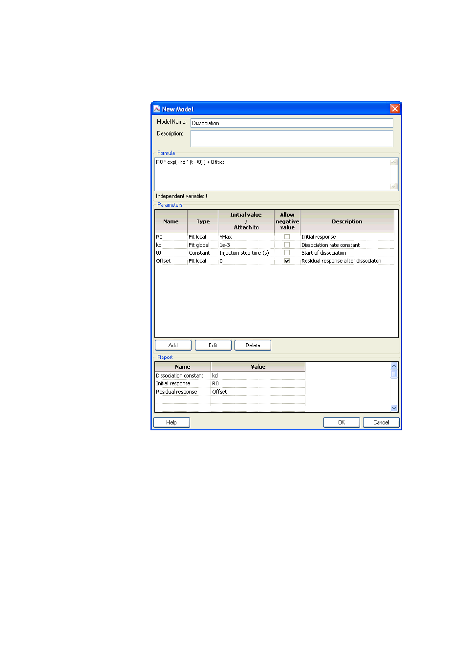
Biacore T200 Software Handbook 28-9768-78 Edition AA 201
Kinetics and affinity analysis 9
The example below shows a model for evaluation of the dissociation phase only.
Parameters and report parameters are defined in the same way as for kinetic
models.

9 Kinetics and affinity analysis
9.9 Creating and editing models
202 Biacore T200 Software Handbook 28-9768-78 Edition AA
9.9.3 Models for steady state affinity
Models for steady state affinity evaluation are entered as an expression
defining R
eq
as a function of concentration Conc. The example below shows a
model for two-site affinity evaluation.
Parameters and report parameters are defined in the same way as for kinetic
models.
Note: Beware of trying to define and use complex models for steady state
affinity. Because of the relatively few points available for fitting to steady
state affinity models (typically about five concentrations in duplicate),
complex models tend to give unstable fitting behavior.

Biacore T200 Software Handbook 28-9768-78 Edition AA 203
Thermodynamic analysis 10
10 Thermodynamic analysis
Biacore T200 supports automated measurement of kinetics or affinity at a
series of temperatures using the Thermodynamics wizard (Section 4.12). In
addition to displaying the variation of kinetic and affinity constants with
temperature, the evaluation software extracts standard thermodynamic
parameters from the data.
10.1 Background
10.1.1 Equilibrium thermodynamics
For equilibrium thermodynamics, the van’t Hoff equation states:
Substituting in the expression
and rearranging gives:
A plot of ln K
D
against 1/T should thus be a straight line, with slope ΔH°/R and
intercept on the y-axis ΔS°/R.
This simplified relationship does not hold if the heat capacities of reagents and
products differ, since different amounts of energy will be required to raise the
temperature by the same amount on the two sides of the reaction. In such
cases, the plot of ln K
D
against 1/T is not linear, and the relationship becomes
where ΔG° is the standard Gibbs free energy change
R is the universal gas constant
T is the absolute temperature (K)
K
D
is the equilibrium dissociation constant
where ΔH° is the standard enthalpy change
ΔS° is the standard entropy change
ΔG° RT
1
K
D
------
ln– RT K
D
ln==
ΔG°ΔH° TΔS°–=
K
D
ln
ΔH°
RT
----------
ΔS°
R
---------
–=

10 Thermodynamic analysis
10.1 Background
204 Biacore T200 Software Handbook 28-9768-78 Edition AA
A value for the standard heat capacity change ΔC
P
° can thus be obtained in
addition to ΔH° and ΔS° from non-linear fitting of the data to this extended
equation.
10.1.2 Transition state thermodynamics
Transition state theory holds that the equilibrium constant for formation of the
transition state in a reaction can be related to the rate constant for the overall
reaction by the Eyring equation:
Applying a similar rearrangement of the thermodynamic equations for the
transition state gives:
so that the thermodynamic transition state constants for the forward and
backward reactions can be obtained from plots of ln(k
a
/T) and ln(k
d
/T)
respectively against 1/T.
Note that the Eyring equation does not have a corresponding non-linear form
that takes account of the heat capacity change for transition state formation.
Non-linear fitting to obtain values for ΔC
P
° can only be applied to equilibrium
thermodynamic analysis.
where ΔC
P
° is the heat capacity change under standard conditions
T
0
is the reference temperature (25°C = 298.15 K for standard
conditions)
where K
‡
is the equilibrium constant for formation of the transition state for
the forward or back reaction
k is the kinetic rate constant for the interaction in the corresponding
direction (k
a
or k
d
)
h is Planck’s constant
k
B
is Boltzmann’s constant
RT K
D
ln ΔH
T
0
°
TΔS
T
0
°
– ΔC
P
°
TT
0
–()TΔC
P
°
T
T
0
-----
⎝⎠
⎛⎞
ln–+=
K
‡
kh
k
B
T
--------
=
kh
k
B
T
--------
ln
ΔH
o‡
RT
-------------
–
ΔS
o‡
R
------------
+=

Biacore T200 Software Handbook 28-9768-78 Edition AA 205
Thermodynamic analysis 10
10.2 Performing thermodynamic analysis
Before thermodynamic analysis can be performed for a set of data, the kinetics
and/or affinity must be evaluated at each temperature. Create a separate
Kinetics/Affinity evaluation item at each temperature used in the run, using the
same fitting model for each item (see Section 9.2).
When all required kinetic and affinity evaluation items have been created, click
Thermodynamics on the toolbar.
Choose the sample and the fitting model in the pull-down lists. You may only
choose one sample, and you should only choose one fitting model. Options for
the model are 1:1 kinetics/steady state affinity (recommended) or All. If you
choose All it is possible to combine data from different fitting models in the
same evaluation: however, values for thermodynamic constants are in all
likelihood meaningless if the data is obtained from a mixture of different models.
Check the rows for data that you want to use in the thermodynamic evaluation.
Use the Check All and Uncheck All as quick options to select and deselect the
whole list.
Note: If you use data from fitting models that include multiple rate or affinity
constants, be sure to select the correct rows so that equivalent constants
are included from each fit. In some cases it may be necessary to examine
the kinetic or affinity evaluation items to determine which constants
belong together.

10 Thermodynamic analysis
10.2 Performing thermodynamic analysis
206 Biacore T200 Software Handbook 28-9768-78 Edition AA
Click Next> when you have selected the data to be included. The results are
displayed first as plots of affinity and rate constants against temperature.
Click Next> to display the van’t Hoff and Eyring plots together with a table of
thermodynamic constants for the equilibrium and transition state formation. In
any of the plots, right-click on a point to exclude the point from the line fitting.

Biacore T200 Software Handbook 28-9768-78 Edition AA 207
Thermodynamic analysis 10
Choose whether to use a linear or non-linear fitting function for the van’t Hoff
plot (see Section 10.1.1). If you choose non-linear fitting, a value for ΔC
p
will be
included in the reported parameters. Energies of activation (E
a
), derived from the
Eyring plots, are also listed for the transition states. All thermodynamic
parameters are calculated for a temperature of 25°C.
In any of the plots, right click on a point to exclude it from the evaluation.
Notes: Regardless of the setting for the van’t Hoff plot, the Eyring plots are
always fitted to a linear function. Calculation of
Δ
C
p
by non-linear fitting
is not valid for transition state data (see Section 10.1.2).
If you have combined kinetic and steady state affinity data in the
thermodynamic evaluation, the van’t Hoff plot will show all affinity values,
but the Eyring plots will be empty because the steady state data lacks
values for the rate constants.
Plots of kinetic and affinity constants against temperature show
temperature values in °C, while van’t Hoff and Eyring plots use absolute
temperature values (K).
Click on Finish to finalize the thermodynamic analysis.
When assessing the validity of thermodynamic constants reported by this
analysis procedure, pay particular attention to the kinetic analysis at different
temperatures. With complex interactions involving macromolecules, there is a
significant possibility that the characteristics of the interaction (including the
role of mass transport limitations in the observed interaction) change with
temperature, resulting in different fitting quality at different temperatures. This
may be evident from direct comparison of the kinetic fits, but will not be
immediately apparent in the thermodynamic analysis.

10 Thermodynamic analysis
10.2 Performing thermodynamic analysis
208 Biacore T200 Software Handbook 28-9768-78 Edition AA

Biacore T200 Software Handbook 28-9768-78 Edition AA 209
Affinity in solution 11
11 Affinity in solution
Determination of affinity in solution provides an alternative to steady state
affinity measurements (see Chapter 9) for interactions that take a long time to
reach equilibrium or for any other reason are difficult to determine with a direct
binding assay. In principle, the affinity in solution approach uses Biacore to
determine the free concentration of one interactant in equilibrium mixtures
containing known total interactant concentrations.
11.1 Conventions and background
11.1.1 Experimental setup
The interactants in affinity in solution determination are denoted A and B:
A + B = AB
Experiments are set up so that a fixed concentration of B is mixed with variable
concentrations of A and allowed to reach equilibrium. The free concentration of
B is then determined by injecting the sample over a ligand that binds B but not
A or the complex AB (the interactant A or a derivative thereof is usually suitable
as ligand). It is assumed that the measurement itself does not significantly
disturb the equilibrium in the sample.
The experimental setup requires a calibration curve with known concentrations
of B determined over the same sensor surface, in order to calculate the free B
concentrations in the samples.
11.1.2 Evaluation principles
The equilibrium constant for a 1:1 interaction is given by
or
K
D
A
free
B
free
⋅
AB
-----------------------------
=
K
D
A
tot
AB–()B
tot
AB–()
AB
------------------------------------------------------- -
=

11 Affinity in solution
11.2 Requirements for affinity in solution
210 Biacore T200 Software Handbook 28-9768-78 Edition AA
Rearranging gives
or
Solving for AB:
Substituting in the relationship B
free
= B
tot
– AB gives
This equation can be fitted to a plot of B
free
against A
tot
to calculate a value for
K
D
. (Formally, the equation has two solutions, but one is always negative and is
not meaningful in the context of an affinity determination.)
11.2 Requirements for affinity in solution
Affinity in solution experiments are run using a method. The method must be
correctly constructed as described in Section 5.10.4: if necessary, the keyword
table can be edited so that the conditions are met in full (see Section 6.6). Note
however that the command type cannot be edited in the keyword table. Refer
to Chapter 5 for details of how to construct methods in Method Builder.
Determination of affinity in solution is not supported by a wizard.
K
D
AB⋅ A
tot
B
tot
AB A
tot
B
tot
+()– AB
2
+⋅=
AB
2
AB A
tot
B
tot
K
D
++()– A
tot
B
tot
⋅+ 0=
AB
A
tot
B
tot
K
D
++()
2
-------------------------------------------
A
tot
B
tot
K
D
++()
2
4
----------------------------------------------
A
tot
B
tot
⋅–±=
B
free
B
tot
A
tot
– K
D
–()
2
------------------------------------------ -
A
tot
B
tot
K
D
++()
2
4
----------------------------------------------
A
tot
B
tot
⋅–±=

Biacore T200 Software Handbook 28-9768-78 Edition AA 211
Affinity in solution 11
11.3 Evaluation of affinity in solution
To evaluate affinity in solution measurements, open the result file and click
Affinity in Solution on the toolbar. The first step displays the calibration curve
for measurement of free B:
Choose the sensorgram, report point, response type and fitting function from
the pull-down lists at the top of the dialog. See Section 8.2.1 for more details of
these choices.
If you have run multiple sample series in the experiment, choose the sample to
evaluate in the Sample list. A sample series is defined as all cycles with the same
sample name in the assay step(s) with purpose Sample.
If you have run multiple calibration curves in the experiment, choose the curve
to use in the Calibration curve list. A calibration curve is defined as
measurements from assay step(s) with purpose Calibration, regardless of the
sample name. If two or more Calibration assay steps are run contiguously with
no intervening steps with a different purpose, they will be combined into a single
calibration curve.
Note: All samples in a series are evaluated against the chosen calibration curve.
You cannot use different calibration curves for different samples in the
same series.
The table lists the data for the calibration curve. The plot panel shows the curve
with calibration points as black inverted triangles and sample points as red
squares. Samples that lie outside the range of the calibration curve are not
shown. Right click on calibration points to exclude the points from the curve.

11 Affinity in solution
11.3 Evaluation of affinity in solution
212 Biacore T200 Software Handbook 28-9768-78 Edition AA
Click Next> to calculate the results.
The table shows the numerical results for the sample series. Samples that lie
outside the range of the calibration curve are marked as N/A (not applicable) in
the column for Calc. Conc. Beq.
The plot panel shows the sample measurements with a line fitted according to
the equation for 1:1 affinity (see Section 11.1.2). Right-click on a point to exclude
it from the fitting.
Notes: The plot of free B against total A is presented by default with a logarithmic
scale on the x-axis.
Zero values cannot be plotted on a logarithmic scale. If you have included
a sample with zero concentration of A in the sample series and want to
display this point on the plot, choose Scale from the right-click menu in
the plot panel and set a linear scale for the x-axis.
The intercept of the fitted curve on the y-axis represents a fitted value for
the parameter ConcB. This value should be the same as or close to the
value entered for the variable ConcB in the method.
The calculated K
D
value is shown in the panel below the table.

Biacore T200 Software Handbook 28-9768-78 Edition AA 213
Immunogenicity 12
12 Immunogenicity
Evaluation of immunogenicity experiments is supported by 4 application-
specific tools in the evaluation software:
• Screening, based on ranking plots for detection of antibody responses.
• Confirmation, for evaluating antibody specificity as tested by inhibition of
responses by added drug. Confirmation evaluation can be based either on
the degree of inhibition by added drug or on a cut-off boundary to classify
inhibition in yes/no terms.
• Isotyping, for identifying positive responses from isotyping reagents.
Isotyping results are presented as bar charts with cut-off boundaries to
exclude negative responses from the chart.
• Stability, which assesses the rate dissociation of detected antibody from
the antigen using a two-site dissociation model.
Evaluation of immunogenicity studies is described in detail in the separate
Biacore T200 Immunogenicity Handbook.

12 Immunogenicity
214 Biacore T200 Software Handbook 28-9768-78 Edition AA

Biacore T200 Software Handbook 28-9768-78 Edition AA 215
Appendices

216 Biacore T200 Software Handbook 28-9768-78 Edition AA

Data import and export Appendix A
Biacore T200 Software Handbook 28-9768-78 Edition AA 217
Appendix A Data import and export
This appendix describes the functions and data format for data import and
export.
A.1 Exporting data
A.1.1 Export functions
Data can be exported from both the Control and Evaluation Software in
Microsoft Excel or Extended Markup Language (XML) format. The report point
table can be exported to a tab-separated text file. Rack positions may also be
exported from the Rack Positions dialog box.
Export to Excel
To export data to an Excel file, choose File:Export:Results to Excel.
Export from the Control Software creates an Excel spreadsheet file (extension
.xls) containing separate worksheets for the file properties and report point
table. The audit trail is also exported to a separate worksheet if it is present
when the GxP module is installed (see the separate Biacore T200 GxP
Handbook).
Export from the Evaluation software an Excel spreadsheet file (extension .xls)
containing separate worksheets for the file properties and for tabulated data
for all evaluation items where appropriate (i.e. plot data and evaluation results).
The worksheets for each item are identified with the item name. For plots, only
the columns shown in the plot window table are exported. Data from
sensorgram items is not exported. The audit trail is also exported to a separate
worksheet if it is present when the GxP module is installed (see the separate
Biacore T200 GxP Handbook).
Export to XML
To export data to an XML file, choose File:Export:Results to XML.
This option exports the same data as Results to Excel but creates a text file in
XML format (file extension .xml). Details of the XML format may be determined
by exporting data from the Control or Evaluation Software and opening the
exported file in an XML-compatible editor.

Appendix A Data import and export
A.2 Importing data
218 Biacore T200 Software Handbook 28-9768-78 Edition AA
Report point table
To export the report point table to a tab-separated text file, choose
File:Export:Report Point Table. The exported file has the extension .rpt.
Note: If you open an exported report point table in Microsoft Excel, make sure
that the format for the Fc column is set to Text in the Excel import file
wizard. The default setting of General for text file import may interpret
the flow cell identification for reference-subtracted data as a date instead
of a text string.
Rack positions
Rack positions can be exported from the Control Software to a tab-separated
text file in either ASCII or Unicode format using the Menu:Export Positions
function in the Rack Positions dialog (Section 4.2.6). The file contains two lines
identifying the microplate and reagent rack settings followed by the contents of
the rack positions table with the columns separated by tabs.
A.2 Importing data
A.2.1 Control Software
The Control Software supports data import to sample tables in assay wizard
templates and in the Setup Run step of methods and to position information to
the Rack Positions step in all runs. In order to use the import function, the option
must be activated in Tools:Preferences and valid import programs must be
specified. Import programs and data files for use with import are the
responsibility of the user.
For each import function, a check box allows the import program to be started
automatically without user intervention. If the respective box is not checked, the

Biacore T200 Software Handbook 28-9768-78 Edition AA 219
Data import and export Appendix A
program will only be started when the user actively requests data import. If the
box is checked:
• Data is imported automatically to the sample table only if the table is
empty. The program is not started if the table already contains data.
• Data is imported to the Rack Positions dialog whenever automatic
positioning is invoked. This happens when the dialog is first opened with
new or modified sample data, and also when the user requests Automatic
positioning from the dialog menu (Section 4.2.6). The program is not
started when the user makes manual changes to the rack positioning or
when the dialog is opened with no changes in previously positioned
samples (for example when the user clicks Back and Next in the dialog
sequence without changing sample information).
Sample table import
When the sample import function is invoked, the contents of the sample table
are first exported in Extended Markup Language (XML) format to a temporary
file that is submitted to the specified import program. The import program may
append new sample data to the file or overwrite the file contents with new data
as required. The modified file is then imported back into the sample table and
the temporary file is deleted.
Development or choice of a suitable import program is the responsibility of the
user. To document the detailed XML format of the import file, specify an XML-
compatible text editor as the import program and save a copy of the import file
from a suitable table.
Figure A-1. Part of an XML import file from a method for heterogeneous analyte kinetics
displayed in an XML-compatible editor.

Appendix A Data import and export
A.2 Importing data
220 Biacore T200 Software Handbook 28-9768-78 Edition AA
Rack positions import
The Menu:Custom Position Import and Simple Position Import functions in the
Rack Positions dialog (Section 4.2.6) import rack position data from an external
file such as one from a laboratory robot used to prepare sample microplates. If
you choose Custom Position Import, the external file is first processed by the
import program as specified in Files:Preferences. Output from this program
must be tab-separated text in either ASCII or Unicode format conforming to the
specification below. The Simple Position Import option imports data from a file
conforming to the specifications with no intervention from an external program.
• Two lines in the file specify the microplate and reagent rack settings, in the
format
Rack1=<microplate specification>
Rack2=<reagent rack specification>
• Specifications are not case-sensitive, but microplate and reagent rack
specifications must be given otherwise exactly as they appear in the
selection lists in the Rack Positions dialog. If either specification is invalid,
the corresponding definition will not be imported. The position of these
two lines in the file does not matter.
• One line specifies the headers for table columns to be imported, separated
by tabs. The headers should correspond to the column headers as they
appear in the Rack Positions table, with the exception of the Volume
column in the table which can be omitted from the import file (and is
ignored if it is present). This line may not be preceded by any line other
than the microplate and reagent rack specifications.
• A set of lines hold the content of the table columns separated by tabs.
Each line must contain the same number of tab characters as the header
line.
When import is requested, the contents of each table line in the import file are
matched as far as possible to the contents of the Rack Positions table, with the
exception of the Position and Volume column. For matched rows, the Position
in the table is replaced by the value in the Position column from the import file.
Rows for which a match cannot be found are not imported. Any rows in the Rack
positions table which do not have a matching row in the import file are left
without a Position specification and must be placed in the microplate or
reagent rack before the run can be started.
Details of the required import file format can be investigated further by
examining a file created with the Menu:Export Positions command.

Biacore T200 Software Handbook 28-9768-78 Edition AA 221
Data import and export Appendix A
Figure A-2. Example of an exported file for rack positions, opened in Microsoft Excel.
A.2.2 Evaluation Software
The Evaluation Software supports import of model definitions for kinetics and
affinity evaluation. Model files for import should be obtained from GE
Healthcare or created by exporting models from another installation.

Appendix A Data import and export
A.2 Importing data
222 Biacore T200 Software Handbook 28-9768-78 Edition AA

Biacore T200 Software Handbook 28-9768-78 Edition AA 223
Method examples and recommendations Appendix B
Appendix B Method examples and recommendations
A selection of predefined methods covering common applications is provided in
the Biacore Methods folder (see Section 5.1). Use these methods either directly
or as starting points for your own method development. This section describes
the essential features in each method that are not supported in wizards. Refer
to these methods as guidelines in constructing your own methods that exploit
similar features.
B.1 Affinity in solution
This method is designed for measurement of affinity in solution as described in
Chapter 11. The method includes a Calibration assay step for measurement of
component B and a Sample step for measurement of mixtures of components
A and B. Both these assay steps are connected to the same cycle type.
Predefined evaluation variables are included for the evaluation purpose Affinity
in solution:
The Variable Settings are different for the two assay steps, so that only the
relevant variables are entered at run-time for each assay step.

Appendix B Method examples and recommendations
B.2 Calibration-free concentration analysis
224 Biacore T200 Software Handbook 28-9768-78 Edition AA
B.2 Calibration-free concentration analysis
Requirements and recommendations for running calibration-free concentration
analysis are provided in this method.
B.2.1 Assay steps and general settings
Blank cycles are run before the samples and are repeated every 12 sample
cycles. Assay steps for samples and blanks are connected to the same cycle
types:
Analysis is performed at a data collection rate of 10 Hz (set in the General
workspace). Do not change this setting.
B.2.2 Cycle types
The cycle type for sample analysis performs a High performance injection with
a contact time of 36 seconds and a dissociation time of 5 seconds. The
dissociation time is not critical: evaluation uses only data from the association
phase. Do not use shorter contact times than 36 seconds, since the actual
contact time (which is determined by the injected volume, rounded to the
nearest µl) may differ significantly at the lowest flow rate.
Sample solution and flow rate are set as method variables. For evaluation
variables, the evaluation purpose is set to Calibration-free conc and predefined
variables MW, D(20°C), Blank and Dilution are required.

Biacore T200 Software Handbook 28-9768-78 Edition AA 225
Method examples and recommendations Appendix B
B.2.3 Variable settings
Sample cycles
All the variables for assay step Sample are set at run time, except for the method
variable Blank which is set to No in the method.

Appendix B Method examples and recommendations
B.2 Calibration-free concentration analysis
226 Biacore T200 Software Handbook 28-9768-78 Edition AA
Blank cycles
For assay step Blank, only the flow rate is set at run time. The method variable
Blank is set to Yes in the method and Sample solution to Buffer. The remaining
variables are not used and may be left blank.
B.2.4 Setup Run
At run time, variables need to be assigned for assay steps Sample and Blank.
Each sample should be run at two or more flow rates: values of 5 and 100 µl/min
are recommended and are entered for one sample. Use the same set of flow
rates for each sample. Values are also required for analyte molecular weight
(MW), diffusion coefficient at 20°C (D(20°C) and dilution factor (Dilution).
Only flow rates are required for assay step Blank: these values must be the
same as the flow rates used for samples.

Biacore T200 Software Handbook 28-9768-78 Edition AA 227
Method examples and recommendations Appendix B
B.3 CAP single-cycle kinetics
This method implements single-cycle kinetics using reversible capture of
biotinylated ligand on Sensor Chip CAP (supported by the Biotin CAPture Kit from
GE Healthcare). This section focuses on the method aspects required for using
the Biotin CAPture Kit. If you want to create a method for other applications
using the Biotin CAPture Kit, modify the Sample cycle definition in the CAP
single-cycle kinetics method. See Section B.10 for aspects of the method
directly related to single-cycle kinetics.
Follow the Instructions for Use supplied with the Biotin CAPture Kit before using
a new Sensor Chip CAP.
B.3.1 Assay steps
The method includes a Conditioning step run once before the start-up cycles.

Appendix B Method examples and recommendations
B.3 CAP single-cycle kinetics
228 Biacore T200 Software Handbook 28-9768-78 Edition AA
This step injects three 1-minute pulses of regeneration solution, and should
always be included at the start of an assay using a new sensor chip. The step
can be omitted if the sensor chip has been used previously.
B.3.2 Sample analysis cycle for Sensor Chip CAP
The cycle definition for sample analysis with Sensor Chip CAP includes 4
injection commands:
• General for injection of the Biatin CAPture reagent
• Capture for injection of the biotinylated ligand
• Sample for injection of analyte
• Regeneration to remove the Biotin CAPture reagent, ligand and bound
analyte

Biacore T200 Software Handbook 28-9768-78 Edition AA 229
Method examples and recommendations Appendix B
An extra wash with buffer after the injection is included in the Regeneration
command.

Appendix B Method examples and recommendations
B.4 GST kinetics
230 Biacore T200 Software Handbook 28-9768-78 Edition AA
B.4 GST kinetics
The recommended method for using a GST-tagged ligand is set up with Dual
detection in General Settings. Detection settings Multi and Single are not
recommended. The method involves 5 conditioning cycles with injection of
recombinant GST (provided in the GST Capture Kit from GE Healthcare) over both
flow cells followed by regeneration:
The sample analysis cycle uses two capture injections, one to capture
recombinant GST on the reference surface only (flow path setting First) and the
second to capture GST-tagged ligand on the active surface only (flow path
setting Second). A stabilization time of 180 seconds is included after capturing
the ligand on the active surface, to allow for dissociation of any weakly bound
components. The sample is then injected over both surfaces. This approach
provides a reference surface that mimics the active surface with respect to
occupancy of the anti-GST capturing sites.

Biacore T200 Software Handbook 28-9768-78 Edition AA 231
Method examples and recommendations Appendix B
This method is set up for kinetic analysis but can be adapted for other assays.
Note: If you change the detection setting to Multi, you will need to include
additional capture injections for the active surfaces in flow cells 3 and 4.
Do not use detection setting Single without removing the first capture
injection.

Appendix B Method examples and recommendations
B.5 Inject and Recover
232 Biacore T200 Software Handbook 28-9768-78 Edition AA
B.5 Inject and Recover
The example method provided for using the InjectAndRecover command is
targeted to recovery for mass spectrometry, and contains two assay steps. The
first conditions the surface by washing three times with 0.5% trifluoroacetic
acid, while the second performs the sample injection and recovery operation.
The cycle for recovery of bound analyte contains just one single
InjectAndRecover command. Additional commands are usually not needed,
since the recovery component of the InjectAndRecover command serves as a
regeneration step (see Section 5.6.1).

Biacore T200 Software Handbook 28-9768-78 Edition AA 233
Method examples and recommendations Appendix B
All parameters in the InjectAndRecover command are fixed: check the
appropriate boxes in the Method Variables list if you want to use variable
parameters. There are no evaluation variables for this command.

Appendix B Method examples and recommendations
B.6 Kinetics heterogeneous analyte
234 Biacore T200 Software Handbook 28-9768-78 Edition AA
B.6 Kinetics heterogeneous analyte
This method is a straightforward kinetics determination with evaluation
variables included for the evaluation purpose Kinetics – heterogeneous
analyte, providing separate concentration and molecular weight variables for
two analytes.
B.7 L1 liposome capture
The recommended method for liposome capture on Sensor Chip L1 uses one
conditioning cycle consisting of two injections of 40 mM octylglucoside, followed
by three start-up cycles using a dummy sample before the actual samples are
run.
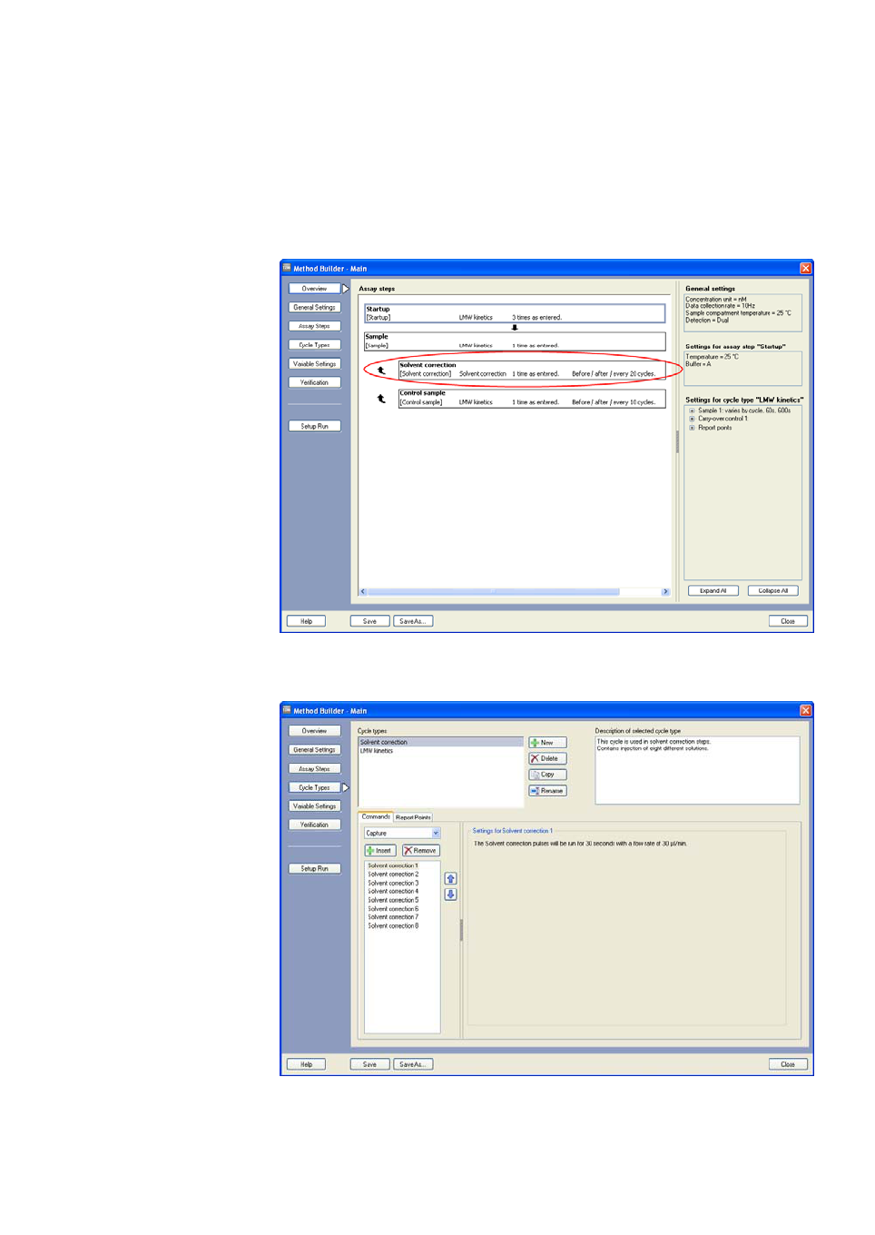
Biacore T200 Software Handbook 28-9768-78 Edition AA 235
Method examples and recommendations Appendix B
B.8 LMW kinetics and LMW Screen
Methods are provided for both kinetics and screening of low molecular weight
compounds. The essential addition to wizard-based counterparts is the
inclusion of a Solvent Correction assay step.
This assay step is connected to a cycle type that includes 8 Solvent Correction
commands for injection of 8 different solvent concentrations (see Section 6.7).

Appendix B Method examples and recommendations
B.8 LMW kinetics and LMW Screen
236 Biacore T200 Software Handbook 28-9768-78 Edition AA
Screening applications suitably include a carry-over control injection, to identify
potential carry-over problems from “sticky” compounds that may affect the
response in subsequent injections. The Biacore method is designed for
screening of low molecular weight compounds and includes a solvent
correction step as described in Section B.8. Low molecular weight compounds
frequently dissociate readily from their targets, and the example method does
not include regeneration. If you require a regeneration step, it is advisable to
include regeneration after both the sample and the carry-over injections.

Biacore T200 Software Handbook 28-9768-78 Edition AA 237
Method examples and recommendations Appendix B
B.9 LMW single-cycle kinetics
This method combines functions for working with low molecular weight
analytes (Section B.8) with the Sample command for single-cycle kinetics
(Section B.10).
B.10 Single-cycle kinetics
The Biacore method for single-cycle kinetics uses the sample command type
Single cycle kinetics with 5 sample concentrations per cycle. Note that with this
command type, the evaluation purpose is fixed as Kinetics/Affinity and the
number of predefined variables for sample concentration corresponds
automatically to the number of sample concentrations per cycle. The
predefined variables cannot be deselected.

Appendix B Method examples and recommendations
B.10 Single-cycle kinetics
238 Biacore T200 Software Handbook 28-9768-78 Edition AA

Biacore T200 Software Handbook 28-9768-78 Edition AA 239
Index
Numerics
1:1 binding 187
A
aborting fitting procedure 166
absolute response 9
, 127, 137
accepting fits 166
active surface 9
adaptive methods 92
adding keywords 115
, 116
adding report points 114
adjust injection start 162
adjustment for controls 132
adjustment for molecular weight 127
affinity 159
, 165, 168
application wizard 65
affinity in solution 95
, 159
evaluation 209
experimental design 209
method example 223
requirements for evaluation 102
,
210
variables 95
aim for immobilized level 41
, 46, 48
aligning sensorgrams 125
alignment 125
analysis temperature 7
, 20, 36, 81, 84
thermodynamics 71
analysis temperature after run 81
analyte 8
, 197
analyte concentration 94
analyte molecular weight 68
, 94
adjusting response 127
anchor 39
append file 108
, 149, 169
application wizards 13
, 29
applying solvent correction 119
assay methods 77
assay setup 32
assay step name 82
assay step purpose 82
, 115
assay steps 78
, 81
analysis temperature 84
buffer change 84
connecting to cycle type 84
recurrence 84
replicates 85
run order 85
auto scale 18
automatic positioning 39
autosampler 62
average calibration curve 141
, 143
avidity 188
B
bar charts 135
display options 136
baseline 96
for report points 96
, 114, 138
in regeneration scouting 52
in sensorgram display 18
plot 112
batch mode 159
, 170
Biacore methods 77
, 223
Biacore terminology 8
BIAnormalizing solution 36
binding analysis 58
results 60
binding capacity 197
binding levels 113
binding partners 58
binding to reference 112
biological significance 184
bivalent analyte 188
blank cycles 95
, 141, 152, 160, 224
blank immobilization 46
blank method 47
blank subtraction 126
, 153, 162
boundaries 134
boundaries for ranking 134
browse buttons 124
buffer 84
buffer bottles 81
buffer change 84
buffer names 81
buffer requirement 41
buffer scouting 54
results 55
buffer selector 7
bulk contribution 117
bulk refractive index 66
, 173, 198
C
calc conc 147
, 155
calculated concentration 146
calculated concentrations 143
calculated parameters 199
calibration curve 61
, 62, 83, 141, 142
calibration curves 211
calibration trends 141
, 144

240 Biacore T200 Software Handbook 28-9768-78 Edition AA
calibration-free concentration
assays 61
, 95, 102, 141, 150, 224
caption 110
capture 31
, 56, 88
flow path 31
plot 112
capturing molecule 8
carry-over control 89
, 236
plot 112
carry-over injection 65
changing rack positions 38
check kinetic data 176
, 178
chip properties 16
, 17, 49
chip type 31
chi-squared 131
, 175
clear positions 38
coefficient of determination 131
coefficient of variation 147
color by 111
, 123, 136
color-coding 37
column labels 136
combined result sets 149
command queue 23
, 25
commands
in manual run 25
in Method Builder 87
competing analytes 189
complex 197
components 177
concentration analysis
application wizard 61
combined result sets 149
evaluation 141
requirements for evaluation 101
,
141
concentration series 68
, 160, 161
concentration unit 81
, 116
conditional command 92
conditional statements 41
conditioning 32
conditioning cycle 83
conformational change 193
connect to cycle type 84
constants 185
contact time 33
, 46
at low flow rates 33
control experiments 73
results 74
control samples 34
, 60, 83, 132
binding analysis 59
concentration analysis 63
, 146
kinetics/affinity 68
plot 112
control software
Edit menu 17
File menu 15
Run menu 19
screen regions 14
Tools menu 19
View menu 18
copy graph 20
, 111
copy table 111
correlated parameters 172
, 177
create
assay step 81
cycle type 86
evaluation method 121
fitting model 195
method 77
wizard template 29
curve 9
, 19
curve fitting 130
, 184
curve name 124
, 128
curve type 171
custom methods for immobilization 47
custom position import 220
custom report points 14
, 95, 113
CV 147
cycle 124
manual run 27
cycle run list 36
, 100
cycle types 78
, 84, 86
D
data collection rate 80
data import 20
data presentation 123
delete
keywords 115
report points 115
deposition solution 90
detecting molecule 61
detection 80
, 98
in wizards 31
diffusion coefficient 95
, 142, 156, 186
diluting ligand for immobilization 46
,
48
dilution factor 64
, 94, 147, 155
dimethyl sulfoxide 66
, 71, 117
dissociation time 59
, 67, 88
disturbed data 154
DMSO 66
, 71, 117
drift 198
dual detection 80
dual inject 91
dummy sample 32

Biacore T200 Software Handbook 28-9768-78 Edition AA 241
E
EDC/NHS 49
Edit menu
control software 17
editing keywords 115
editing report points 115
in control software 17
in evaluation software 113
eject chip 20
, 27
eject rack 20
, 24, 27
manual run 26
ending a manual run 27
enhancement 31
, 56, 89
plot 113
enthalpy 203
entropy 203
epitope mapping 58
estimated buffer requirement 41
estimated run time 41
evaluating concentration analysis 141
Evaluation Explorer 108
evaluation items 108
evaluation methods 121
evaluation of kinetics and affinity 159
evaluation procedures 121
evaluation purpose 93
, 171
evaluation requirements 101
evaluation software
general features 107
screen regions 107
evaluation variables 93
, 115
event log 14
, 19
event markers 19
, 126
Excel 217
excluded cycles 143
excluded volume effect 118
excluding data
from concentration analysis 143
,
147, 148
from evaluation 110
from kinetics/affinity
evaluation 162
from plots 129
expand all cycles 150
expected concentration 63
, 147
export 15
export curves 20
, 111
export rack positions 40
export to Excel 217
export to XML 217
exporting data 217
exporting plots 111
exporting rack positions 40
, 218
exporting the report point table 218
extra wash after injection 87
extrapolating solvent correction
curves 121
Eyring equation 204
F
File menu
control software 15
file name extensions 21
file storage 21
filter keywords 116
filtering report point table 138
fit by color 130
fitting curves to plots 130
fitting function 142
, 144
fitting models 148
, 157, 166, 171
fitting parameters 166
, 168
flow cell 7
, 9, 45, 80
flow path 80
, 98
for buffer scouting 54
for capture 31
in wizards 30
manual run 24
, 26
method runs 98
flow rate 33
, 46, 141, 151, 186
effect on binding rate 73
manual run 24
, 26
range 33
folder for methods 77
folder for wizard templates 29
four-parameter fit 62
, 131, 144
free energy 203
G
general command 91
general settings 80
global parameters 168
, 185
gridlines 21
, 111
group by 136
GST Capture Kit 230
GST-tagged ligand 230
GxP compliance 8
H
heat capacity 204
heterogeneous analyte 94
, 189
method example 234
heterogeneous ligand 191
high performance injection 88
, 91
I
if...then command 92
immobilization 45
methods 45

242 Biacore T200 Software Handbook 28-9768-78 Edition AA
results 49
immobilization pH scouting 42
import program 219
import rack positions 40
importable wizard templates 77
importing rack positions 40
, 220
importing sample tables 59
, 64, 68,
99, 218
importing wizard templates into Method
Builder 77
included blanks 153
initial values 199
inject and recover 90
, 232
inject sample
manual run 26
injection parameters 33
injection sequence 30
injection volumes 33
injections 31
, 87
insert chip 20
instrument preparation 23
instrument preparations for manual
run 23
interaction kinetics 159
interaction models 196
interpolated calibration 141
K
keyword table 14
, 115
kinetic constants 172
kinetics 159
, 165
predefined models 186
kinetics control experiments 73
kinetics/affinity
application wizard 65
calculated values 168
evaluation 159
requirements for evaluation 102
,
160
subsets 169
kinetics/affinity report 168
k
m
186
k
t
186
L
labels in plot windows 110
legend 111
ligand 8
, 197
ligand capture 31
ligand immobilization 45
limit guides 179
linear fit 131
, 144
linked reactions 73
control experiment 73
control results 75
liposome capture 234
local parameters 168
, 185
lock scale 18
low molecular weight compounds 235
low sample consumption 88
, 91
LRSD 138
M
main screen
control software 14
evaluation software 107
maintenance tools 20
manual run 13
, 23
initial settings 24
markers 126
mass spectrometry 7
, 90
mass transfer 73
, 179, 197
control experiment 73
control results 74
mass transfer coefficient 186
mass transfer constant 176
, 186
mass transfer parameters 186
mass transport limitation 151
measured conc 155
menus 14
Method Builder 13
, 77
commands 87
importing wizard templates 77
method examples 223
method files 21
method overview 78
, 79
method structure 78
method variables 93
methods 77
assay 13
evaluation 121
folder 21
, 77
microplate 23
, 38, 39
in manual run 24
Microsoft Excel 217
mix 61
, 89
in concentration analysis 61
mix and inject 48
mixing sample before injection 89
modification factor 178
molar concentrations 68
molecular weight 142
of analytes 68
multi detection 80
multi-component complex 58
multi-cycle kinetics 65
, 159
multiple data sets 162
multiple ligand densities 169

Biacore T200 Software Handbook 28-9768-78 Edition AA 243
evaluation 170
multiple result files 108
multiple R
max
162, 169
N
nested assay steps 81
new cycle in manual run 27
normalize 36
normalizing sensorgram display 125
notebook 19
, 21
O
octylglucoside 234
opening files for evaluation 108
optimum buffer pH 44
optimum immobilization pH 44
orientation 39
overview 79
P
parameter significance 176
parameters button 171
parameters for kinetics/affinity 166
pausing a manual run 27
pH range 43
pH scouting 42
results 44
plot windows 127
fitted curves 130
table columns 129
polynomial fitting 132
pooling 39
preconcentration 42
, 43, 46, 48
predefined
evaluation items 112
evaluation variables 93
immobilization methods 45
methods 77
, 223
models 186
plots 112
predip 87
preferences 40
, 77
prepare run protocol 41
prime 19
, 36
print layout 16
print range 16
printing rack positions 40
printing results 16
, 109
printing wizard templates 40
Q
QC ratio 151
acceptance 151
quality control 167
, 172
queue 23
, 25
R
rack 39
rack illumination 20
rack positions 37
automatic import 40
default positions 38
export 40
, 218
import 40
, 220
rack settings in manual run 24
ranking 134
rate equations 199
, 200
reactants 196
reagent rack 23
, 38, 39
recovering bound analyte 90
recovery solution 91
recurrent assay steps 84
reference line 18
reference subtraction 118
, 126
reference-subtraction 9
regeneration 9
, 31, 34, 89
manual run 26
regeneration conditions 51
regeneration scouting 50
results 52
regeneration solutions
viscosity 26
, 34, 51, 89
regions 39
regression coefficient 138
regulated environments 8
relative response 9
, 114, 127, 138
reliability of K
D values
195
remove selection 164
removing data from sensorgram
display 124
renaming keywords 117
repeat calibration 62
replicate assay steps 85
replicate concentrations 62
report point id 114
, 137
report point markers 19
report point range 121
report point table 14
, 21, 136
export 218
report point window 114
, 137
report points 9
, 95, 113, 136
adjustment for molecular
weight 127
editing in control software 17
in regeneration scouting 52
markers 126
R
eq against C
165
requirements for evaluation 101

244 Biacore T200 Software Handbook 28-9768-78 Edition AA
requirements for kinetics and affinity
evaluation 160
residual analyte 65
residuals 168
, 174
resonance unit 9
response bound 49
response correction factor 190
response type 127
result files 21
right-click menu 20
, 25, 99, 109
Run menu
control software 19
run order 68
, 85
run protocol 41
run time 97
running buffer 84
running wizards 30
S
sample capacity 7
sample command 88
sample compartment
illumination 20
temperature 7
, 36, 71, 80, 84
sample concentrations 68
sample injection 31
, 34
binding analysis 58
sample mixing in concentration
analysis 61
sample name in calibration curve 144
sample names 162
sample parameters
binding analysis 59
sample response
in regeneration scouting 52
samples 34
for calibration curve 62
for concentration analysis 64
for kinetics/affinity 68
scale 18
, 20, 109, 111
screen regions
control software 14
evaluation software 107
screening 58
method example 236
SD 138
selecting data for thermodynamic
evaluation 205
selector bar 15
, 124, 128
selector button 124
Sensor Chip L1 234
Sensor Chip SA 48
sensor chip type 31
sensorgram 9
adjustment 125
baseline 18
copy graph 20
curvature 173
display 123
export curves 20
, 111
in evaluation 123
markers 19
normalizing 125
printing 16
reference line 18
removing data for display 124
window 14
service tools 20
settings for regeneration scouting 51
settings for R
eq
165
setup run 98
short-term noise 174
show sensorgram 110
shutdown 19
significance 176
simple position import 220
simulate cycle run list 82
single detection 80
single-cycle kinetics 65
, 88, 159, 161,
237
slope 138
sodium acetate buffers 43
software help 15
solvent correction 66
, 71, 83, 90, 117
applying 119
extrapolation 121
method example 235
principle 119
requirements for evaluation 103
solvent correction curves 120
fitting 120
shape 121
slope 121
sort keywords 116
sorting
plots 130
report point table 138
specifying variable values 97
SPR technology 7
stabilization period 87
, 89
stabilization time 34
standard deviation 138
standard error 176
standby 19
start-up cycles 32
, 83
in regeneration scouting 50
statistical parameters 175
status bar 14
, 108

Biacore T200 Software Handbook 28-9768-78 Edition AA 245
steady state affinity 165, 195, 202
stop command in manual run 27
stop run 27
subset 169
surface performance 56
results 57
system caption 110
system overview 7
system preparations 35
, 100
T
table
in plot windows 129
table columns 129
target immobilization level 46
t
c
186
temperature 20
, 23, 36
temperature control 7
temperature dependence of kinetics
and affinity 206
temperature equilibration 41
, 71
template types 29
templates 29
folder 21
, 29
importing into Method Builder 77
terminology 8
test tools 20
thermodynamic parameters 203
thermodynamics 159
application wizard 70
evaluation 203
requirements for evaluation 102
tool tips 123
toolbar 14
Tools menu
control software 19
transition state 204
T-value 176
two-state reaction 193
U
uniqueness 172
, 177
unknown samples 141
unzoom 18
, 109, 111
user-defined caption 110
user-defined variables 93
using calibration trends 145
U-value 177
V
van’t Hoff equation 203
variable settings 97
variables 78
, 93, 97, 115, 127
entering values at run time 98
entering values in a method 97
verification 79
, 98
vial size 39
view curve 19
View menu
control software 18
viscosity 26
, 34, 51, 89
W
wait
manual run 26
weight-based concentrations 68
window 96
, 114
wizard components 30
wizard results 19
wizard templates 29
, 77
wizards 13
, 29
importing into Method Builder 77
work area 108
X
XML 217
, 219
Z
zero concentration samples 68
, 160,
162
zero response point 125
zero time point 125
zoom 18
, 109
zoom lock 53
, 109

246 Biacore T200 Software Handbook 28-9768-78 Edition AA


28-9768-78 AA 05/2010
For contact information for your local office,
please visit
www.gelifesciences.com/contact
GE Healthcare Bio-Sciences AB
Björkgatan 30
751 84 Uppsala
Sweden
www.gelifesciences.com/biacore
GE and GE monogram are trademarks of General Electric Company.
Biacore is a trademark of GE Healthcare companies.
All third party trademarks are the property of their respective owners.
© 2010 General Electric Company—All rights reserved.
First published May 2010
All goods and services are sold subject to the terms and conditions of sale
of the company within GE Healthcare which supplies them. A copy of these
terms and conditions is available on request. Contact your local GE
Healthcare representative for the most current information.
GE Healthcare UK Ltd
Amersham Place, Little Chalfont, Buckinghamshire, HP7 9NA, UK
GE Healthcare Bio-Sciences Corp
800 Centennial Avenue, P.O. Box 1327, Piscataway, NJ 08855-1327, USA
GE Healthcare Europe GmbH
Munzinger Strasse 5, D-79111 Freiburg, Germany
GE Healthcare Bio-Sciences KK
Sanken Bldg. 3-25-1, Hyakunincho, Shinjuku-ku, Tokyo 169-0073, Japan
