1 Our Changing Forests Level 2 Graphing Exercises (Google Sheets

Our Changing Forests Level 2 Graphing Exercises (Google Sheets)

In these graphing exercises, you will learn how to use Google Sheets to create a simple

pie chart to display the species composition of your plot, a bar graph to compare the DBH

of all trees in a plot, a histogram to look at the frequency at which trees of different

species appear at different sizes, and another bar graph to compare trees in two different

sites.

Exercise 1 - Pie Chart

Goal: To create a pie chart to show the composition of tree species in the Applewild

(AWH) Our Changing Forests plot.

1. Download data from the Applewild School (AWH) from the HF Schoolyard

online database into a new spreadsheet in Google Sheets. You can either save the

data to your desktop and open the file in Google Sheets, or you can open the data

in Excel and copy and paste it into Google Sheets.

Schoolyard LTER database > download data > choose school > submit >

download data > save .csv file and open in Google Sheets

Schoolyard LTER database > download data > choose school > submit >

download data > open .csv file in Excel (generally the default program) > copy

and paste into Google Sheets

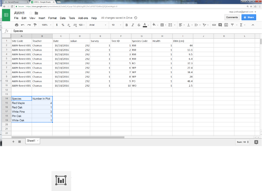
2. Create a new table from the data to describe what you want to graph. In this case,

we want to make a graph showing how many of each different tree species we

have in our plot. I’ve pulled from the downloaded data to make a new table that

contains only the data I want to graph right now.

3. Highlight the data in the new table (including the headers) and click the insert

chart icon on the toolbar.

4. Make sure the data is being displayed in a pie chart. Pie charts are usually the

best type of graph to make when you want to display the pieces of a whole. So in

this case, we want to show that even though our plot contains different types of

trees, when you add them up, they make up 100% of the trees in the plot. Also,

make sure the graph has a title. In this chart editor screen you can change lots of

things regarding how the pie chart works. Play around! You can always start over

if you make something you don’t like.

5. If you’ve made a mistake or realize there’s something you want to change after

you’ve inserted your graph, you can click the arrow in the top right-hand corner

of the graph to make edits. You can also move the graph to a better location on

the spreadsheet, save the image, or copy and paste it into another document. Once

you’ve pasted the graph somewhere else, you won’t be able to edit it.

Exercise 2 - Bar Graph

Goal: To create a bar graph to compare the DBH of each tree in the Applewild Our

Changing Forest plot.

1. Working from the same downloaded data set, you will again need to pull from the

existing data to make a table that describes what you want to graph. In this case,

we’re going to be graphing each tree’s DBH measurement. Keep in mind that

however you choose to label each tree in the data table is how it will be

represented on your graph. Instead of the tree IDs 1, 2, 3 etc., I wanted my trees to

be labeled with their species.

2. Highlight the table and pick the kind of chart you want using the insert chart

button. We want a column chart (bar graph).

3. Edit the graph to your liking. I added a title, changed the color of the bars,

changed the size of the axis labels and changed the maximum measurement on the

y-axis to 50 cm so that you could better see the bars.

Exercise 3 - Histogram

Goal: To create a histogram to compare the frequency at which each type of tree occurs at

different size classes at one field site in the Groton-Dunstable High (GDH) Our Changing

Forest study.

A histogram is similar to a bar graph in that the data are represented in bars. However, in

a histogram, the bars depict counts so that you can analyze the frequency at which a

variable occurs. So in this case, we are going to be looking at how many small, medium

and large trees there are in one plot.

1. Download the GDH data from the database into a new datasheet. GDH has

multiple sites and data collected in multiple years, but we’re just going to use the

most recent data from site 2, collected on 6/9/16 because there are a lot of trees.

Everything else can be omitted.

2. Sort your data. Similarly to the other two exercises, the first thing we are going to

do is make a table with exactly the data we want to graph. However, making a

table for a histogram is a little more challenging than the other tables we’ve made

so first, we’re going to sort the data to make it easier to use. To start, highlight

your entire data set. Right click the box at the upper left corner of the

spreadsheet. A drop down menu will appear with a "Sort range" option. Select it

and sort by appropriate column(s).Ultimately we are going to be organizing this

chart by species.

3. When making a table for a histogram in Google Sheets, the top left most box

needs to remain blank at all times. The way you want to bin (or group) your data

goes in the first column and will appear on the x-axis. In this case, we want to bin

our data by DBH class. Tree species will go along the top of the table because in

this histogram, each bar is going to represent a different type of tree. Finally, the

number of trees of each species in each DBH class go inside the table because we

are interested in the distribution of this variable. I found it easier to just type each

value into the boxes by hand, but you can also copy and paste.

I also found it easier to color-code the trees in the dataset by DBH class so that I

could more easily find the values I needed for my table.

4. Highlight the new data table and insert a chart. Make sure you choose a

histogram. You might have to play around with some of the initial settings. Make

sure the switch rows/columns box is unchecked. Edit the graph so that each axis is

labelled, the scale along the y-axis is appropriate and the graph has a title.

Exercise 4 – Scatterplot

Goal: To create a multi-site scatterplot to describe the relationship between the number of

trees in each field site and the total basal area of the site.

1. For this scatterplot, we will be looking at a large data set because we are

comparing the trees at different schools. Go to the database and download all of

the data from the 2016 field season. The following schools submitted data in

2016: AWH, BCE, DFA, GDH, GUM, HAE, HBH, MHH, SHH, WAM. The

easiest way to get all of this data is to download the data for all sites. Then, in

Google Sheets, sort the data by ‘Date’ (See Exercise 3 for how to sort data.) Then

delete data for years other than 2016.

2. Create a new column after DBH (cm) and label it Basal Area.

3. Write a function to compute the basal area of each tree. If DBH is the length of

the diameter of the tree, basal area is the area of each tree if you were to take a

cross-section, or a slice of the trunk. We assume the cross-section of the trunk is a

circle, so the area of this cross section = pi*radius

. To find basal area, we use the

formula BA=0.00007854*(DBH)^2 where BA is the basal area of a tree in square

meters per hectare and DBH is the diameter of the tree at breast height in

centimeters.

To write a function, you must first start with an = because that tells Google Sheets

that you are going to be writing a formula. In your new basal area column, write

the formula =0.00007854*(DBH^2), but instead of DBH, you’re going to click

the DBH measurement in cell I2. This tells Google Sheets that you want to use

that value in your equation.

4. Compute the basal area for every tree in the dataset. Luckily for you, you don’t

need to write a new function for every line of data. You can just drag the bottom

right-hand corner of the cell we just used down the entire spreadsheet. Google

Sheets knows to reference the adjacent value in the I column to compute the

appropriate basal area.

5. Compute the total basal area for each field site. We have just found the basal area

for each tree in the dataset, and now we need to add those up for each field site to

get the total basal area. Again, we’re going to write a function in any empty cell.

To sum things, Google Sheets uses the =SUM(BA) function. However, instead of

BA, you’re going to highlight all of the BAs in one of the school field sites. (A

quicker, but more advanced, way to do this is to use a Pivot Table.)

6. Calculate the number of trees in each field site. If you recall, this scatterplot is

graphing the total basal area of a plot against the number of trees in that plot.

Input the number of trees in each plot somewhere on the spreadsheet that will be

easy for you to reference later.

7. Make a table. By now you should be pretty good at this! Make a table at the

bottom of your spreadsheet that contains the total basal area and the number of

trees for each school.

8. Match your units. The formula for basal area gives a value in m

per hectare,

however, the number of trees in each plot is number of trees per 100m

because

each plot is 10m x 10m. To make the graph easier to interpret, we want all of our

units to be in hectares. A hectare is 10,000m

, so we need to multiple each of

number of trees per plot values by 100 to get the number of trees per hectare. You

could do this by hand, or by using a function.

9. Make your scatterplot. Highlight the data in your table and insert a scatterplot.

10. Don’t forget to label your axis and your graph, and to adjust your scale if

necessary.

11. If you want the color of each dot to be coded for a site, you have to format the

data table differently. You still have one column for Number of Trees, but the

Basal Area data for each site gets its own column, with the Site name as the

column heading.

12. Each column then becomes a ‘Series’ when making the graph.

What conclusions, if any, can we draw from this graph? Is this graph what you

might expect to see when comparing the total basal area of a plot to the number of

trees in that plot? Can you think of any variables that may be affecting the data

besides the ones we have graphed?

Alternate Exercise 4 - Multi-Site Bar Graph

Goal: To create a bar graph showing the correlation between DBH of maple trees in a

hillside upper field site and a dry flat field site.

Because we don’t yet have many years worth of data to look at, it may be more

interesting to make cross-site rather than multi-year comparisons. For one thing, you only

need one year of data to compare two (or more) different sites.

1. Download your data. For this exercise, we are going to use data from both

Applewild (hillside upper) and Groton-Dunstable (dry flat), so you will need to

have both of these data sets downloaded side by side in one spreadsheet. Even

though GDH has multiple sites with several years of data, I am only going to use

the most recent data available -- site 2 which was sampled on 6/9/16. Everything

else can be omitted.

2. Build your table so that you have DBH along the y axis and field site along the x

axis. Each bar will represent a tree. Remember, we are just looking at the

difference between the DBH of red maples between these two sites in one year.

3. Insert a bar chart from your data table and edit the chart to your satisfaction.

While interesting to look at, it’s impossible to say from this chart that the type of

field site (dry flat versus hillside upper) is the only reason that the AWH maple

trees appear to have a larger DBH on average than the GDH maples. Can you

think of any other reasons why the maple trees in these two sites might differ?

Further Practice

Want to keep practicing? Here are some more ideas of ways you can graph your OCF

data. Which graph do you think would best illustrate these relationships? Keep in mind

that, especially when looking at the change in DBH over time, we may not yet have

enough data to make these graphs.

• How many trees are dead or alive in the plot?

• How much space (basal area) does each species take up in the plot?

• Compare growth (DBH) between members of one species

• Compare species composition between two different plots

• Compare growth (DBH) of one species between multiple schools

• Compare growth (DBH) of one species between multiple schools across multiple

years

• Compare species composition (or DBH) between two schools with the same site

survey description components (landscape position, slope, canopy cover etc.)

• Compare species composition (or DBH) between two schools with different site

survey components (landscape position, slope, canopy cover etc.)