Insurers Monitor Shocks to Collateral: Micro Evidence from

Insurers Monitor Shocks to Collateral:

Micro Evidence from Mortgage-backed Securities

∗

Thiemo Fetzer

University of Warwick and Bonn & CEPR

Benjamin Guin

Bank of England

Felipe Netto

Bank of England

Farzad Saidi

University of Bonn & CEPR

August 30, 2024

Abstract

This paper uncovers if and how insurance companies react to shocks to collateral in

their portfolio of securitized assets. We address this question in the context of commercial

real estate cash ﬂow shocks, which are informationally opaque to holders of commercial

mortgage-backed securities (CMBS). Using detailed micro data, we show that cash ﬂow

shocks during the COVID-19 pandemic predict CRE mortgage delinquency, especially

those stemming from lease expiration of oﬃces, reﬂecting lower demand for these prop-

erties. Insurers react to such cash ﬂow shocks by selling more exposed CMBS—mirrored

by a surge in small banks holding CMBS—and the composition of their CMBS portfolio

aﬀects their trading behavior in other assets. Our results indicate that institutional in-

vestors actively monitor underlying asset risk, and even gain an informational advantage

over some banks.

JEL codes: G20, G21, G22, G23

Keywords: Insurance Sector, Risk Management, Mortgage Default, Commercial Real Es-

tate, CMBS, Work-from-home

∗

We thank David Glancy, Thorsten Martin, Ralf Meisenzahl and Lakshmi Naaraayanan, as well as seminar

participants at Queen Mary University of London, University of Leicester, the 2024 BEAR Conference at the

Bank of England, and the 2024 Conference on Regulating Financial Markets at Frankfurt School of Finance

& Management for helpful comments. Saidi acknowledges funding by the Deutsche Forschungsgemeinschaft

(DFG, German Research Foundation) under Germany’s Excellence Strategy (EXC 2126/1 – 390838866) and

through CRC TR 224 (Project C03). Fetzer acknowledges funding by the Leverhulme Prize in Economics, a

European Research Council Starting Grant (ERC, MEGEO, 101042703), and Deutsche Forschungsgemeinschaft

(DFG, EXC 2126/1 – 390838866). The paper represents the authors’ personal opinions and not necessarily the

views of the Bank of England.

1. Introduction

Growing risks in mortgage-backed securities, along with perceived failure by intermediaries

to perform due diligence and risk management, are considered some of the main causes of

the Global Financial Crisis (Chen et al., 2020). For commercial mortgage-backed securities

(CMBS), such risks arise due to the uncertainty about cash ﬂows generated by the underlying

mortgages. Yet, monitoring these cash ﬂows is particularly challenging in CMBS as these

securities often contain several underlying assets and complex structures (Ghent, Torous and

Valkanov, 2019). By studying how investors react to salient shocks to (expected) cash ﬂows,

we can infer whether they monitor such risks in complex assets.

In this paper, we exploit cash ﬂow shocks during the COVID-19 pandemic that vary by the

type of property serving as mortgage collateral. Retail properties faced shocks due to lock-

downs, leading immediately to signiﬁcantly lower revenue. By contrast, the shift to hybrid

work arrangements reduced demand for oﬃce spaces, thereby aﬀecting their current and ex-

pected revenue and value (Gupta, Mittal and Nieuwerburgh, 2023). This poses additional

challenges to CMBS investors’ monitoring eﬀorts. Moreover, the extent to which investors

diﬀer in their due diligence and risk-bearing capabilities also determines how commercial

real estate (CRE) risks associated with lower oﬃce demand are shared across intermediaries.

Speciﬁcally, we explore how insurers—one of the largest investor groups in mortgage-

backed securities—react to increases in CRE mortgage risks induced by cash ﬂow shocks both

during COVID-19 and in its wake. To this end, we exploit rich data on mortgages included

in CMBS deals, containing detailed loan and property characteristics, as well as information

about the lease contracts between borrowers and their core tenants. Lease expiration has a

strong positive eﬀect on CRE loan default for oﬃces, especially following the COVID-19 pan-

demic, when demand for oﬃce real estate dwindled as a result of hybrid work arrangements.

We present evidence in line with the view that insurers monitor collateral characteristics such

as property type and lease expiration dates, and reduce their holdings of CMBS exposed to

these risks after the onset of the pandemic. Moreover, the composition of insurers’ CMBS

portfolio has implications for how these investors react to salient risks in the remainder of

their asset portfolio. Finally, we document how the reduction in CMBS holdings by insurers

is accompanied by a signiﬁcant increase in the holdings of private-label CMBS in particular

by small banks.

We start out by discussing the link between borrower cash ﬂows obtained from rental in-

come and mortgage delinquency, and how this information would inﬂuence CMBS investors’

behavior depending on monitoring. Since the value of a commercial property equals the

present discounted value of the cash ﬂows that can be obtained from renting such property,

changes in cash ﬂows and changes in property value are intimately connected. Lower de-

mand for CRE would aﬀect delinquencies through their eﬀect on cash ﬂows obtained from

renting out properties, and risks to these cash ﬂows are more likely to materialize once a ten-

ant agreement ends. Importantly, if lease agreement information is monitored by investors,

then these investors would be more likely to sell CMBS with a larger share of mortgages

linked to leases expiring when faced with unexpected shocks to collateral demand. More-

over, this monitoring eﬀort could make investors less reactive to risks in other assets if their

capacity to monitor such risks is limited.

To test the relationships between information about CRE cash ﬂow risks, loan delinquency,

and institutional investors’ trading behavior, we use comprehensive monthly panel data on

CMBS deals, bonds and loans against CRE, along with detailed information on the asset

portfolios of U.S. insurance companies. The mortgage data enable us to observe the default

status of each loan while also capturing relevant information about the underlying proper-

ties, including their location and designated use. The dataset also contains rental contract

characteristics such as lease expiration dates and tenant occupancy share for certain types

of properties. Following our discussion, we posit that changes in rental cash ﬂows are more

common when tenant lease contracts expire, since elevated early termination fees can incen-

tivize tenants to retain their lease until it expires.

The lease expiration timing generates

a negative cash ﬂow shock for borrowers if they need time to ﬁnd a new tenant or if they

cannot renew the lease at a similar rent. Indeed, we ﬁnd spikes in delinquency that coincide

with months in which the lease contracts of borrowers’ main tenants expire, especially for

oﬃces, rendering the monitoring of lease expirations potentially valuable.

We next turn to diﬀerences in default for properties with and without leases expiring, be-

fore and after the COVID-19 pandemic. The underlying rationale is that cash ﬂow shocks

This should hold true under the condition that the costs of terminating the rental contract early are higher

than the savings from moving to a smaller oﬃce space.

should be stronger following a systematic drop in demand for commercial real estate. The

COVID-19 period is characterized by structural changes in demand for oﬃce space due to

hybrid working arrangements (Barrero, Bloom and Davis, 2021). Lower demand for oﬃces

reduces current and expected rental income, lowering the value of commercial real estate

properties. We show evidence consistent with the presence of a structural shift in demand for

oﬃce space, leading to more persistent increases in mortgage defaults, especially for mort-

gages exposed to lease expiration.

The challenge in establishing a causal link between lease expiration dates and delinquency

rates is that these dates can coincide with other shocks that cause delinquency. For example,

lease expiration can coincide with regional shocks that lower demand for CRE. Similarly,

if mortgages with leases expiring have ﬂoating interest rates, increases in reference interest

rates that coincide with lease expiration can also cause an increase in delinquency rates. We

address these challenges by leveraging the granularity of our data, which allow us to include

a rich set of ﬁxed eﬀects that capture several static and time-varying confounding factors

that could aﬀect delinquency rates.

Using the beginning of the COVID-19 pandemic as the treatment period of a shock to the

demand for oﬃce space, we estimate a diﬀerence-in-diﬀerences speciﬁcation, and show that

lease expiration triggers increases in delinquencies, with a stronger eﬀect after COVID-19.

These eﬀects are economically meaningful, with lease expiration leading to about 1.3 per-

centage points higher delinquency in the baseline period, and an additional 1.2 percentage-

point increase in the post-pandemic period. Finally, the lease expiration eﬀect is stronger

for properties which are not fully occupied by the largest tenants, suggesting that relatively

larger tenants renew their leases more often.

The second step in our empirical analysis consists of understanding how large insurance

companies’ exposure to oﬃces through their CMBS holdings are, and the extent to which

these investors monitor cash ﬂow risk caused by lease expiration. First, we document that in-

surance companies are indeed a large group of investors in CMBS, holding close to one-fourth

of newly issued private-label CMBS between 2017 and 2022. We also ﬁnd that the amount

of insurers’ private-label CMBS portfolio not exposed to oﬃces peaks in 2020, and decreases

afterwards, which is consistent with lower demand for CMBS exposed to oﬃces among those

investors. Nonetheless, insurers remain largely exposed to cash ﬂow risks arising from lower

oﬃce demand. In our sample, the median insurance company has its private-label CMBS

with an average exposure of about 26% to oﬃces. This potentially dwarfs banks’ exposure to

other CRE-related risks, often of indirect nature (Acharya et al., 2024).

We test if insurers monitor cash ﬂow risks in their CMBS portfolio by asking if bonds more

sensitive to diﬀerent cash ﬂow shocks are more likely to be sold following the sudden, un-

expected increase in risk caused by COVID-19. Our identiﬁcation strategy relies on the idea

that pandemic-driven lower demand for CRE constitutes an unexpected shock to CMBS cash

ﬂows, with diﬀerent eﬀects across property collateral types. As with mortgage default, we

estimate a diﬀerence-in-diﬀerences speciﬁcation to assess if CMBS with exposure to oﬃce-

linked loans whose main leases expire within a speciﬁc horizon are more likely to be sold

after the pandemic. The richness of our data allows us to include insurer by time and insurer

by bond ﬁxed eﬀects, on top of time-varying coupon type and risk classiﬁcation ﬁxed eﬀects.

This addresses concerns that our estimates are contaminated by other time-varying insurer

shocks or bond characteristics. Moreover, it allows us to capture changes in trading behavior

within an asset class with similar capital costs for insurers.

We ﬁnd that insurers infer risks from shocks to expected cash ﬂows, aﬀecting their trading

behavior. Insurance companies are more likely to sell CMBS which are exposed to oﬃces,

especially those with lease expiration in the medium term. Insurers are also more likely to

sell retail-exposed CMBS, but this eﬀect is not sensitive to underlying lease expiration. This

suggests that insurance companies can identify how diﬀerent property types are aﬀected by

the pandemic, and the nature of cash ﬂow risks caused by lower demand for oﬃces. Further-

more, medium-term lease expiration in four to six years has strong predictive power for sales

of oﬃce-linked CMBS. For instance, bonds exposed to oﬃce lease expiration within six years

are over two percentage points more likely to be sold by insurers in the post-COVID period.

Their sensitivity to underlying lease expiration in longer horizons indicates that the market

expects a whole asset class—commercial real estate—to be aﬀected by the pandemic shock

for a longer duration.

Insurers adjust to risks in CMBS also along other margins. First, the share of CMBS ac-

quired by insurers with oﬃce exposure falls after 2020, along with the share of CMBS ex-

posed to cash ﬂow shocks via lease expiration. Second, insurers demand higher coupons for

holding oﬃce-exposed CMBS originated after the pandemic, even when controlling for other

determinants of CMBS returns. These ﬁndings corroborate the idea that insurers monitor

risks to their CMBS portfolio, and learn about structural changes that make certain types of

collateral more prone to cash ﬂow-induced losses.

We also consider aﬀected insurers’ trading behavior in the remainder of their securities

portfolio. As insurers react to immediate losses in retail-exposed CMBS, this could trigger

sales of other risky assets (Ellul et al., 2022). Indeed, we ﬁnd that insurance companies are

more likely to sell risky assets if they have a larger exposure to retail collateral. At the same

time, insurers put in eﬀort to assess underlying risks in their portfolio of securitized assets

as they become more relevant, as was the case for oﬃce-linked CMBS during the COVID-

19 pandemic. By locking down valuable monitoring eﬀorts, this gives rise to the possibility

that insurance companies are subsequently less sensitive to increases in capital requirements

or other consequences of holding on to riskier assets in the remainder of their portfolio.

Consistent with this, we ﬁnd that insurers are less likely to sell riskier bonds in the post-

COVID period if they have a larger exposure to oﬃces in their CMBS portfolio, even when

controlling for time-varying unobserved heterogeneity at the insurer and security level. The

latter eﬀect points to the limited resources that ﬁnancial institutions have at their disposal to

eﬀectively constrain their exposure to investment with lurking risk (e.g., Chen et al., 2020).

If insurers reduce their exposure to private-label CMBS, other investors are acquiring these

risky assets. Since monitoring of securitized assets is costly, it is possible that less sophisti-

cated investors are less sensitive to lurking risk and end up holding larger shares of private-

label CMBS after the pandemic. In line with this view, we document a remarkable rise in the

holdings of private-label CMBS by banks after 2020, especially by small and medium-sized

banks. The number of small banks that hold private-label CMBS nearly doubles between 2020

and 2023. Since small banks are in general not exposed to large oﬃce-linked loans (Glancy

and Kurtzman, 2024), this could be caused by additional risk-bearing capacity. However,

to the extent that small banks have lower risk management abilities (Ellul and Yerramilli,

2013), this is also consistent with the idea that better informed insurers oﬄoad part of their

oﬃce-borne CMBS risks to less well informed small banks. Moreover, contrary to insurers,

other investors do not seem to demand higher coupons from oﬃce-exposed CMBS after the

pandemic, suggesting these investors are indeed less sensitive to such risks. Our ﬁndings

point to how investors’ ability to monitor risks in complex assets contributes to the transfer

of risks caused by systematic shocks.

Related literature. Our paper contributes to the literature studying securitized assets and

mortgage-backed securities in particular.

This literature has pointed out to how risks in

mortgage-backed securities (MBS) aﬀected institutional investors during the Global Finan-

cial Crisis. Several papers investigate how MBS characteristics such as equity retention (Be-

gley and Purnanandam, 2017) and retention structure (Flynn, Ghent and Tchistyi, 2020)

are used by originators to signal asset quality. Ghent, Torous and Valkanov (2019) show

how more complex CMBS underperform during the Global Financial Crisis, with complexity

contributing to both obfuscating collateral quality and allowing for cash ﬂows to be diverted

towards residual tranches. Moreover, investors do not price this complexity-induced default

risk. These studies emphasize the diﬃculty in assessing risks in MBS, which requires costly

infrastructure to be performed (Hanson and Sunderam, 2013). Our contribution is to show

that despite these due-diligence challenges and being typically viewed as less capable of

doing so, institutional investors monitor detailed, time-varying property and lease contract

characteristics that predict CMBS losses, and divest on the basis of such information.

As such, our paper also relates to a broad literature that studies insurance companies’

portfolio decisions, and how they react to risks in their asset portfolio.

This literature doc-

uments that insurance companies react to changes in observable risk such as downgrades

(Ellul, Jotikasthira and Lundblad, 2011), and highlights how regulation aﬀects insurers’ be-

havior facing asset risk (Chen et al., 2020; Becker, Opp and Saidi, 2022; Sen, 2023). We

contribute to it by showing how insurers divest from CMBS with larger cash ﬂow risks fol-

lowing the pandemic, even if these risks do not immediately lead to higher capital costs.

Moreover, in line with Ellul et al. (2022), we ﬁnd that insurers divest from risky assets when

a large share of their CMBS portfolio suﬀers a devaluation shock, and that the additional

eﬀort undertaken to monitor those cash ﬂow risks seems to limit insurers’ ability to react

to salient risks in other assets. This ﬁnding is particularly relevant given the importance of

insurance companies in absorbing ﬂuctuations in asset prices (Chodorow-Reich, Ghent and

See, for example, DeMarzo and Duﬃe (1999), DeMarzo (2005), Demiroglu and James (2012), Ashcraft,

Gooriah and Kermani (2019), and Aiello (2022).

See, among others, Ge and Weisbach (2021), Koijen and Yogo (2022), Bretscher et al. (2022), Bhardwaj, Ge

and Mukherjee (2022), and Koijen and Yogo (2023).

Haddad, 2021).

Finally, we relate to the literature exploring the impact of work-from-home adjustments

in CRE mortgage default risk. Thus far, this literature had not documented a direct link

between lower oﬃce demand and CRE mortgage default (Nieuwerburgh, 2022).

Moreover,

Jiang et al. (2023) explore how losses from CRE loan portfolios aﬀect the solvency of U.S.

banks, and Glancy and Kurtzman (2024) considers how diﬀerences in small banks’ CRE loan

portfolios govern reduced exposure to loans whose poor performance was driven by lower

oﬃce demand. Our contribution is to provide a detailed account of how insurers are aﬀected

by CRE risks through their CMBS holdings. Moreover, variation in how insurers react to

shocks expected to materialize in diﬀerent horizons suggests market participants expect the

oﬃce demand shock to have a long duration. Finally, the exposure of small banks to CRE

risks through their holdings of CMBS has been largely ignored so far. As CRE risks shifted

across the ﬁnancial sector, the number of small banks exposed to CMBS has increased sub-

stantially. In that sense, any comprehensive analysis of how CRE risks will aﬀect ﬁnancial

stability should account for both banks’ and non-banks’ CMBS exposures alike.

2. Lease Expiration, Cash Flow Shocks, and CRE Mortgage Default

In this section, we develop hypotheses that will guide our empirical analysis. First, sudden

drops in demand for oﬃce space lead to fewer occupied oﬃces after leases expire, either

by downsizing or lack of renewal, and longer search times for new tenants. This results in

lower income from new leases, reducing overall lease revenue. As a result, to the extent that

borrowers rely on such income to repay mortgages, mortgage default rates should increase,

especially in periods of lower demand for oﬃce space.

Hypothesis 1: Lease expiration persistently increases defaults of mortgages against oﬃces after the

COVID-19 cash ﬂow shock, whereas other types of collateral, especially retail, see defaults imme-

diately and are, thus, less sensitive to lease expiration.

As in our study, Glancy and Wang (2024) highlights the importance of lease expiration in the post-COVID

period, showing that it aﬀects oﬃce vacancies and loan performance. Both studies provide direct evidence

of the importance of cash ﬂow-triggered mortgage default for commercial real estate. Several papers study

the relevance of strategic and cash ﬂow motives for default of residential mortgages (Ganong and Noel, 2023;

Bhutta, Dokko and Shan, 2017; Gerardi et al., 2018), with less attention devoted to commercial mortgages.

Since U.S. insurers frequently hold CMBS, any increase in the riskiness of these assets

could inﬂuence their investment decisions. First, if insurance companies can observe lease

expirations, the increased likelihood of future delinquencies due to lease expirations should

make CMBS with a higher proportion of soon-to-expire mortgages less attractive to hold.

Since lower demand increases the persistence of default triggered by lease expiration, in-

vestors are more likely to monitor characteristics associated with cash ﬂow risks following

the pandemic-linked shock to CRE demand. Consequently, they are more prone to selling

CMBS with a larger exposure to cash ﬂow shocks after the pandemic.

Hypothesis 2: Conditional on monitoring, insurers should sell CMBS with relatively more mort-

gages against oﬃces undergoing lease expiration after the COVID-19 cash ﬂow shock, while their

propensity to sell CMBS with retail exposure increases immediately and is otherwise invariant to

the horizon of lease expiration.

Mortgage-backed securities are complex assets, assessing risks for these assets is costly and

often accessible only to sophisticated institutional investors (Hanson and Sunderam, 2013).

Even if insurers possess the ability to monitor the cash ﬂow risks associated with lower CRE

demand and lease expiration, as hypothesized, other intermediaries might not. In that case,

if insurers sell CMBS with a larger exposure to cash ﬂow risks, and if intermediaries diﬀer

in their monitoring capacity, the sale of CMBS by insurers would be accompanied by an in-

crease in the holdings of less sophisticated investors.

Hypothesis 3: If monitoring capacity is heterogeneous, risky CMBS should, on average, ﬂow from

insurers to less sophisticated investors.

Finally, the demand shock for oﬃce space leading to an unexpected increase in cash ﬂow

risks to CMBS portfolios can aﬀect insurers’ trading activity in other assets. This is possible

for two reasons. First, facing immediate losses—as is the case for retail-exposed CMBS—in

their asset portfolio caused by higher delinquencies after the onset of the pandemic, insur-

ers might de-risk by selling other, riskier assets (Ellul et al., 2022). Moreover, if insurance

companies’ risk assessment capacity is limited (Chen et al., 2020), insurers which exert more

eﬀort to monitor cash ﬂow risks—especially those linked to oﬃce collateral—to their CMBS

portfolio after the onset of the COVID-19 pandemic could become less sensitive to conse-

quences of holding riskier assets. This reduction in the salience of risk characteristics for

other bonds in insurers’ portfolios would lead to lower sales in response to changes in ob-

servable risk, such as rating downgrades or capital surcharges.

Hypothesis 4: Insurers’ holdings of CMBS aﬀect their trading behavior in other risky assets diﬀer-

ently depending on the type of collateral.

3. Data Description

Our data come from two main sources: Trepp and the National Association of Insurance

Companies (NAIC). Trepp is a lead provider of commercial real estate collateralized prod-

ucts data, which is established in the existing literature (Flynn, Ghent and Tchistyi, 2020).

It collects origination information from CRE mortgages, CMBS deals and bonds, which is

obtained from various sources. It includes detailed information such as property type and

location, mortgage maturity, amount, interest rates, and delinquency information for each

distribution date. We classify loans according to the use of the property which serves as col-

lateral for the loan. We distinguish between Oﬃce, Retail, and further property types.

The

data also contain information on lease agreements between borrowers and tenants. We focus

on the lease information for the largest tenant only. Appendix-Table A.1 shows that the avail-

ability of lease expiration data varies by property type, with Oﬃce and Retail as the only two

property types for which the date of lease expiration of the main tenant is available for more

than 50% of the observations. For this reason, we mainly consider these two property types

throughout the paper.

We obtain holdings and trades of ﬁxed income assets of all insurance companies in the

U.S. from the National Association of Insurance Commissioners (NAIC). The holdings data

These are classiﬁed as Multifamily, Mixed Use, Healthcare-Nursing, Lodging-Restaurants, Industrial and Ware-

houses, and Other. The details of how these types are obtained, along with other details of our data cleaning

procedure, can be found in Appendix B.

are based on NAIC Schedule D Part 1, and contain CUSIP-level end-of-year holdings of ﬁxed

income securities, including CMBS. The trading information is obtained from NAIC Sched-

ule D, Parts 3 and 4, which contain information on acquisitions and dispositions of ﬁxed

income assets by insurance companies, respectively. We identify actual trades (sales and

purchases) using a procedure similar as in Becker, Opp and Saidi (2022), which is described

in Appendix C.

We restrict our analysis to the post-2017 period.

This ensures that we mitigate concerns

about the inﬂuence of the Global Financial Crisis (GFC), e.g., through elevated delinquency

rates responding to demand shocks that originated during the GFC. Table 1 shows the sum-

mary statistics of the mortgages in our sample. Panel A focuses on all properties, which have

a median lease expiring in 2024 and a median mortgage maturity of 10 years. We classify a

loan as delinquent if payments are past due for at least 90 days. On average, less than 1% of

all loans are delinquent in our sample period, around 10% of our loans have ﬂoating interest

rates, and less than 1% are recourse loans.

Finally, since our analysis mostly focuses on oﬃces and retail CRE, we provide a break-

down of the characteristics of the mortgages used to ﬁnance these property types in Panels B

and C of Table 1, respectively. Relative to retail, oﬃces have ﬂoating interest rates more fre-

quently, lower delinquency rates, and similar maturity. Moreover, the mean and the median

share of each property occupied by the largest tenant is smaller in oﬃces than in retail.

4. Cash Flow Shocks and Mortgage Delinquencies

4.1. The Role of Lease Expiration

First, focusing on mortgages whose lease expiration dates occur between 2017 and 2021,

we evaluate the importance of lease expiration-induced cash ﬂow shocks to borrowers in

driving delinquency rates. Using this sample period, we examine delinquency rates in the

time window of one year prior and one year after the expiration date of the main lease. Given

our deﬁnition of a loan being delinquent if it is at least 90 days, or about 3 months, past due,

we expect to see delinquency rates to increase comparatively more only after the third month

Our Trepp sample covers CMBS information until June 2022.

in which a lease expires.

Figure 1 shows the average delinquency rates for all property types for which such in-

formation is available. As expected, we observe that delinquency rates increase, with the

sharpest increase occurring exactly in the fourth month after the lease expiration date. This

is in line with the idea that cash ﬂow shocks from a lease expiring induces borrowers to

stop making payments on their mortgages. This may be because the existing borrower can-

not ﬁnd a new tenant immediately or the lease generates lower income than the previous

one. Moreover, delinquency rates seem to converge back to their pre-lease expiration trend

approximately 10 months after the lease expiration, which indicates that borrowers resume

their payments once a new tenancy agreement is secured. This further illustrates the impor-

tance of cash ﬂow shocks to the default behavior of CRE borrowers.

This preliminary analysis, however, does not account for potential diﬀerences in delin-

quency rates depending on the use of the property. There are reasons to assume that such

diﬀerences exist. First, the speciﬁc use of the property might limit a borrower’s ability to

ﬁnd a new tenant. For example, it may be more diﬃcult to re-purpose oﬃce space for other

uses, which can increase search costs and lower expected revenue after an existing lease ex-

pires. Second, ﬁrms in diﬀerent sectors might be more likely to renew their lease contracts,

and to the extent that these ﬁrms select into diﬀerent types of properties, this would dif-

ferentially aﬀect borrowers depending on the property they are ﬁnancing with their loan.

Third, it may be borrower-speciﬁc characteristics that matter. For example, some borrowers

who take out mortgages against certain types of properties might struggle more to ﬁnd new

tenants, which would be the case if search frictions are diﬀerent when looking for oﬃce or

retail tenants. Against this background, we split our sample into two subsamples: oﬃces

and other retail properties. Figure 2 shows a remarkable diﬀerence in delinquency behavior

for these diﬀerent property types. The plot on the left-hand side shows sharp increases in

delinquency rates of oﬃces following the end of the main lease agreement. By contrast, the

plot on the right-hand side suggests that increases in delinquency rates of retail properties

are more short lived, with shocks introduced by the end of lease agreements being more tran-

sitory in nature. Overall, these preliminary results indicate that cash ﬂow shocks are strong

predictors of oﬃce delinquencies, but less so for retail properties.

So far, we have examined delinquencies focusing on the exact timing of the lease expiration

for a speciﬁc property, but not explicitly considering the delinquency behavior of mortgages

without leases expiring. This diﬀerence in exposure to cash ﬂow shocks caused by lease

expiration can be particularly relevant in the post-COVID period, as lower demand for oﬃces

could interact with these contractual terms and lead to more persistent losses to landlords. To

the extent that lower CRE demand magniﬁes cash ﬂow shocks, one would expect mortgages

with leases expiring in the post-COVID period to perform worse than mortgages which are

not subject to such cash ﬂow shocks.

We assess diﬀerences in delinquency of properties with and without leases expiring by

looking at oﬃce/retail properties for which we have lease expiration information (i.e., we

know if the main lease expires or not), and zoom in on the immediate period before/after

the start of the COVID-19 pandemic. We compare the average delinquency rate of loans

with leases expiring in 2021-2022 with the average delinquency rates of loans without leases

expiring in these two years.

The results are shown in Figure 3. The left-hand side plot shows a remarkable pattern for

oﬃce mortgages with and without leases expiring in 2021-2022. Delinquency rates for the

former group are pretty much stable throughout the entire period, whereas there is a large

spike in delinquency rates for mortgages the main leases of which expired in 2021-2022. This

further indicates that cash ﬂow shocks are a relevant determinant of oﬃce mortgage default,

and that aggregate delinquency rates do not capture the extent to which work-from-home

arrangements trigger CRE mortgage default given its eﬀect on oﬃce demand.

By contrast, the trajectory of retail mortgage delinquencies on the right-hand side of Figure

3 shows a diﬀerent pattern. Delinquency rates spike immediately at the onset of the COVID-

19 pandemic, which coincides with lockdown periods during which retail stores did not

generate income to tenants. Following that initial shock, mortgages with leases expiring

in 2021-2022 demonstrate persistently higher delinquency rates. which suggests that lease

expiration matters for the adjustment to the initial shock. In other words, while cash ﬂow

shocks do not seem to cause mortgages to go from performing to non-performing in the case

of retail, they do seem to aﬀect the persistence of the initial increase in delinquency rates.

In what follows, we focus on oﬃces rather than retail properties. This allows us to focus

on structural changes in the demand for oﬃce space without explicitly considering the im-

plications from the initial lockdowns on businesses. Furthermore, if institutional investors

trade before losses materialize, then one would expect their trading behavior to be based on

oﬃce exposure if these mortgages losses can be predicted by shocks to expected cash ﬂows.

4.2. The Eﬀect of Lease Expiration on Mortgage Delinquency

Our motivating evidence suggests a key role for lease expiration dates in driving delinquency

behavior for CRE mortgage borrowers, especially for oﬃce properties. Nevertheless, there

are a range of other factors that could be driving the delinquency dynamics we observe for

properties subject to lease expiration. For example, lease expiration dates could correlate

with systematic or region-speciﬁc shocks that aﬀect the U.S. economy in speciﬁc times, such

as the Global Financial Crisis and the onset of the COVID-19 pandemic. Moreover, loans for

which we have lease expiration data could also have speciﬁc characteristics, such as ﬂoating

interest rates, which can make them more susceptible to increases in delinquency in times of

increases in interest rates.

To evaluate the relationship between lease expiration and mortgage default, we leverage

the richness of our data, which allow us to compare otherwise similar mortgages that have

leases expiring and not. First, we estimate the following speciﬁcation:

D90

jrt

= α

+ α

j(f loating)t

ι∈[−15,15]\{0}

+ ε

jrt

, (1)

where I

D90

jrt

is an indicator variable equal to 1 if loan j, for a property located in city r, is

delinquent for more than 90 days in month t, D

equals 1 if loan j is ι months after lease

expiration in month t. α

and α

are loan and city-year ﬁxed eﬀects, which allow us to control

for time-invariant loan-level and time-varying regional characteristics that might inﬂuence

default rates. α

j(f loating)t

are interest rate type by year ﬁxed eﬀects to capture diﬀerences in

delinquency between ﬂoating and ﬁxed interest rate loans.

The coeﬃcients of interest δ

capture the percent diﬀerence in delinquency rates ι months

before and after lease expiration, relative to the moment in which the lease expires. Impor-

tantly, the use of comprehensive ﬁxed eﬀects ensures this variation does not correspond to

time-varying regional shocks or to index rate characteristics of the mortgages that could also

inﬂuence delinquency behavior. We only include loans for which we have lease expiration

information

, and cluster standard errors at the loan level.

Since lower oﬃce demand caused by work-from-home (WFH) arrangements might aﬀect

CRE mortgage default rates, we estimate (1) separately for the period before and after the

COVID-19 pandemic started (where we consider March 2020 as the beginning of the pan-

demic). Intuitively, if borrowers face lower demand for their properties as a result of struc-

tural changes associated with work-from-home preferences, then one would expect the cash

ﬂow shocks introduced by lease expiration to be long lasting. Conversely, absent demand

shocks, the initial drop in cash ﬂows would cease after the borrower manages to ﬁnd a new

tenant, and delinquency rates would slowly transition back to their pre-lease expiration lev-

els.

The results are shown in the two plots of Figure 4, indicating that WFH demand adjust-

ment did aﬀect the persistence of the eﬀect of cash ﬂow shocks on delinquency rates. While

the initial eﬀect is similar in both periods, delinquency rates in the pre-COVID panel on

the left show that delinquency rates begin to converge back to their initial level after one

year of the lease expiration. Our point estimates indicate that relative to the lease expiration

month, a mortgage experiences a one percentage point higher delinquency 15 months after

the lease expiration. In contrast, the eﬀects of the cash ﬂow shock induced by lease expiration

are more long lasting in the post-COVID period, with delinquency rates gradually becoming

larger following a lease expiration. The diﬀerence in relative delinquency between the lease

expiration month and 15 months after is about three percentage points, almost three times

as the same point estimate from the pre-COVID period.

To quantify the diﬀerences in post-lease expiration delinquency behavior before and after

the onset of the COVID-19 pandemic indicated in Figure 4, we estimate a triple-diﬀerences

speciﬁcation:

We do this to avoid including loans with leases expiring in our control group (which could happen for loans

for which we do not observe that information, but might experience a lease expiration nonetheless).

D90

jrt

= α

+ α

j(f loating)t

+ γ

P ost Expiration

+ β

P ost Expiration

× P ost Covid

+ β

P ost Expiration

× Ind Of f ice

+ β

P ost Covid

× Ind Of f ice

+ β

P ost Expiration

× P ost Covid

× Ind Of f ice

+ ε

jrt

, (2)

where P ost Covid

is a dummy equal to 1 after March 2020, P ost Expiration

equals 1 if

loan j had its main lease expiration before or in month t, and Ind Of f ice

equals 1 if loan j

is linked to an oﬃce. The coeﬃcient of interest β

captures the diﬀerence in the eﬀect of lease

expiration-induced cash ﬂow shocks on delinquency rates since the onset of the pandemic.

The results are shown in Table 2. Across all speciﬁcations, the coeﬁcient on the triple

interaction term is positive and statistically signiﬁcant, and the economic magnitude is rele-

vant. The baseline eﬀect of lease expiration on mortgage delinquency increases by about 1.2

percentage points, meaning the eﬀect of cash ﬂow shocks on delinquency rates is twice as

strong after the COVID-19 pandemic. Cash ﬂow shocks increase delinquency rates by more

than 2 percentage points when compared to the average delinquency rate of 0.6% for prop-

erties without expired leases in the post-COVID period. This is an economically signiﬁcant

eﬀect, with delinquency rates of oﬃce mortgages whose main tenancy agreement expired

being more than four times as large as delinquency rates of mortgages that do not experi-

ence such cash ﬂow shocks. These results reinforce the notion that demand shocks caused

by hybrid work arrangements, which became prevalent after the beginning of the COVID-19

pandemic, further exacerbate the eﬀects of cash ﬂow shocks on CRE mortgage delinquency

rates.

CMBS exposure to regional work-from-home characteristics. Our analysis hinges on the

observation that by being relatively more aﬀected by hybrid work arrangements, demand

for oﬃce properties is also relatively more aﬀected by the work-from-home shock, thereby

leading to more persistent cash ﬂow shocks to rent revenue. Importantly, another dimension

of heterogeneity in exposure to work-from-home adjustments refers to regional characteris-

tics. For instance, cities like San Francisco or New York are perceived to be more aﬀected by

hybrid work arrangements than others (Gupta, Mittal and Nieuwerburgh, 2023).

While we cannot measure demand for oﬃce space, we can nevertheless assess how mort-

gages in our sample correlate with measures that have been constructed to capture regional

sensitivity to work-from-home. We use the measure of jobs that can be performed remotely

by Dingel and Neiman (2020), which should broadly indicate which areas are more likely to

be aﬀected by work-from-home arrangements. Figure A.3 in the Appendix shows the distri-

bution of the percentage of teleworkable jobs in an MSA, for the oﬃce-linked mortgages in

our sample and for all MSAs. Relative to the distribution across all MSAs, oﬃce-linked mort-

gages in our sample are located in areas with higher sensitivity to work-from-home shocks.

4.3. Cash Flow Shocks and Relative Tenant Occupancy

Our results so far focus on the sensitivity of default rates along the extensive margin of lease

expiration—namely, whether a lease expiring is associated with increases in default—but is

silent about the intensive margin—i.e., whether the relative size of an occupant also aﬀects

default. On the one hand, tenants which occupy a larger share of a property might also

have more bargaining power and obtain better renewal oﬀers, rendering them more likely to

renew their contracts. On the other hand, since these tenants also represent a larger share of

the rental income obtained from a property, unexpected vacancy would have a larger impact

on borrower cash ﬂows.

We investigate these opposing forces by analyzing how our lease expiration results interact

with tenant occupancy. Figure A.2 shows that Oﬃces and Retail CRE have similarly shaped

distributions of the percentage occupied by a property’s largest tenant. In both cases, there is

substantial mass at 100%, with around 16% of the tenants occupying the whole rental unit.

For that reason, we re-estimate (2) and split our sample between mortgages whose underly-

ing properties are fully occupied by the largest tenant and those with partial (below 100%)

occupancy. Additionally, we estimate a version of (2) using the entire sample and adding an

additional interaction term with Full

, which equals 1 if a property is fully occupied by its

largest tenant in month t.

Table 3 shows the results, with columns 1 to 3 focusing on properties fully occupied by

the largest tenant, columns 4 to 6 partially occupied by the largest tenant, and columns 7

to 9 with the additional interaction term using the whole sample. Consistent with the idea

that relatively larger tenants have more bargaining power and obtain more favorable condi-

tions for renewing, we observe that both the baseline eﬀect of lease expiration and the post-

pandemic diﬀerential eﬀect of cash ﬂow shocks to Oﬃce CRE mortgage default are stronger

for properties partially occupied by the largest tenant. This further indicates that character-

istics of the underlying tenancy agreements of properties ﬁnanced by securitized mortgages

are important for CMBS cash ﬂows.

5. Do Insurers Monitor Cash Flow Risks?

We have documented a signiﬁcant link between expected changes in the tenancy agreement

of a speciﬁc oﬃce and default rates of the mortgage linked to that property, which has im-

plications for assets whose cash ﬂows depend on the performance of these CRE mortgages.

In particular, insurance companies’ cash ﬂows obtained from their holdings of CMBS might

be compromised if the underlying mortgages become non-performing. This raises several

fundamental questions. What is the extent and dynamics of the exposure of insurance com-

panies to oﬃce CRE through their holdings of CMBS? Moreover, given the predictable nature

of expected cash ﬂow shocks to mortgage payments, do insurance companies monitor such

risks and sell bonds based on such cash ﬂow shocks to mortgage CRE? Finally, does lower

oﬃce demand introduced by work-from-home preferences in the post-pandemic period af-

fect the trading behavior of these intermediaries? We explore the answers to these questions

next.

5.1. Insurer Holdings of WFH-sensitive CMBS

We start by leveraging our data to document the importance of insurance companies for the

private-label CMBS market, and to characterize their exposure to shocks linked to oﬃce col-

lateral. We are in a unique position to do so, given our access to detailed CMBS information

(including origination dates) and granular data on the portfolio of insurance companies.

First, we collect information on end-of-year outstanding balances and amounts issued for

all private-label CMBS in our sample, and identify which bonds are held by insurance compa-

nies at the end of each year. Figure 5 shows that insurance companies are the main investors

in CMBS markets. By the end of 2022, insurance companies hold about $600 billion out of

$800 billion outstanding. Similarly, between 2017 and 2019, insurance companies acquired

more than 70% of the total amount of new issues of private-label CMBS. Interestingly, the

share of new CMBS originations held by NAIC insurers in the same year drops to about 65%

between 2020 and 2022. This reduction in the overall amount of CMBS held by insurance

companies is indicative of lower insurer demand, which could arise as lower oﬃce demand

leads to mortgage default rates.

We further explore how the dynamics of CMBS holdings by insurance companies varies

over time, by documenting the exposure of insurance companies’ CMBS portfolio to oﬃce

CRE collateral. We classify a bond as exposed if it has any mortgages ﬁnancing oﬃce prop-

erties within its pool of collateral. We then calculate the share of CMBS that is exposed to

oﬃces out of the entire portfolio of private-label CMBS held by insurance companies. Figure

6 shows the share invested in non-exposed bonds for each year. One can see that the share

of CMBS exposed to oﬃces increases up until 2020, at which point this trend is reversed. In

particular, insurance companies increase the share of CMBS not exposed to oﬃces in 2021

and 2022 by about ﬁve percentage points. This further suggests insurers reacted to risks

arising from lower demand for oﬃce space by adjusting their holdings of CMBS.

Next, we document the exposure of insurance companies to risks related to expiring ten-

ancy agreements of mortgage-ﬁnanced oﬃce properties. We calculate the percent share of

mortgages against oﬃces in each deal associated with a CMBS bond in our sample, for all of-

ﬁces, as of June 2022. We also compute the share of this portfolio of oﬃce-linked CMBS with

underlying leases expiring between 2023 and 2026. Intuitively, this percentage represents

how exposed to oﬃce mortgages a particular bond is, abstracting from seniority consider-

ations. Figure 7 shows the resulting distributions. The left plot considers exposure to any

oﬃce properties, while the right plot considers exposure to oﬃce properties with at least one

underlying mortgage with a tenancy agreement expiring between 2023-2026. The median

insurance company has its private-label CMBS with an average exposure of about 26% to of-

ﬁce properties, and 4.6% to oﬃce properties with tenancy agreements expiring in 2023-2026.

Importantly, there is considerable heterogeneity in the size of the average exposure of CMBS

bonds to oﬃce properties among insurance companies, with the top decile of the distribution

of insurers with an average exposure of 39% of their portfolio to oﬃces, and 10% to oﬃces

with underlying lease expiration.

5.2. CMBS Exposure to Cash Flow Shocks and Trading Behavior

We next exploit exposure heterogeneity across insurers to estimate its eﬀect on insurers’ trad-

ing behavior. Insurance companies might anticipate the eﬀect of work-from-home (WFH)

shocks on the cash ﬂows and on the value of their CMBS, and attempt to sell these bonds.

Moreover, even if insurance companies do not trade CMBS based on oﬃce exposure alone,

they could still anticipate shocks to their assets caused by upcoming lease expiration.

First of all, it is instructive to understand if investors observe and trade based on the un-

derlying characteristics of mortgages included in CMBS. In particular, to the extent that lease

expirations predict delinquency rates, insurance companies might attempt to oﬄoad exposed

CMBS in anticipation of losses associated with default. Moreover, this information might be

less salient to other market participants, which could put insurance companies in a unique

position to trade at more advantageous conditions than when default risk materializes. To

test this, we estimate the following speciﬁcation:

sold

ijt

= α

+ α

j(coupon)t

+ α

j(NAIC)t

+ β

Y Of f ice

+ ε

, (3)

where I

sold

ijt

is a dummy variable which equals 1 if insurer i actively sold any fraction of

security j in year t.

and I

Y Of f ice

are indicator variables capturing two measures of

exposure Y , lease expiration within one year and delinquency rates, for all properties and

only oﬃces, respectively. α

and α

denote insurer-year and insurer-security ﬁxed eﬀects.

We also include interest type by year ﬁxed eﬀects α

j(coupon)t

and NAIC designation by year

ﬁxed eﬀects α

j(NAIC)t

, to capture time-varying willingness to trade bonds with ﬁxed interest

rates or diﬀerent credit ratings. We use exposure to lease expiration in the following year

and exposure to underlying delinquency in the current year. Intuitively, these results should

indicate whether insurers are more likely to sell bonds which are currently underperforming,

or are expected to underperform, in the following year. Standard errors are clustered at the

security level.

The results are shown in Table 4. One can see that only realized, but not expected, un-

For details on how this variable is constructed, see Appendix C.

derlying losses trigger CMBS sales by insurance companies. Importantly, while most of the

variation in realized losses (columns 3 and 4) comes from oﬃce properties, the variation in

expected losses does not depend on property types. This is consistent with the notion that

insurance companies’ selling decisions generally depend on losses to the underlying collat-

eral having actually materialized. This suggests that they do not, on average, monitor bond

performance as related to pending risks.

The work-from-home shock leads to a revaluation of oﬃce properties, however. There-

fore, if insurance companies have the capacity to monitor such risks once they become more

salient, we would expect them to react to expected losses only after the onset of the COVID-19

pandemic.

To explore this possibility, the second step in our analysis is to shed light on whether in-

surance companies anticipate demand adjustments due to work-from-home shocks, which

became prevalent with the pandemic. The WFH transition reduces uncertainty regarding

which types of real estate will be aﬀected by realized and expected shocks. This provides in-

surance companies with the opportunity to anticipate which CRE assets will be most aﬀected

by demand-induced cash ﬂow shocks, and to potentially trade before losses materialize. To

understand if insurance companies trade based on expected cash ﬂow shocks, we test if they

sell private-label CMBS with larger exposure to oﬃce mortgages with leases expiring in dif-

ferent time horizons more frequently after the pandemic started. Formally, we estimate the

following speciﬁcation:

sold

ijt

=α

+ α

j(coupon)t

+ α

j(NAIC)t

+ β

P ost Covid

× I

Exp(τ)

+ β

P ost Covid

× I

ExpOf f ice(τ)

+ β

P ost Covid

× I

Of f ice

+ ε

ijt

, (4)

where P ost Covid

equals 1 after 2019, I

Exp(τ)

and I

ExpOf f ice(τ)

are dummies which equal

1 if bond j is exposed to mortgages whose main lease expires within t + τ years (excluding

year t), for all properties and only oﬃces, respectively. We do not include delinquent loans

when creating the lease expiration treatment dummies, as to avoid capturing the eﬀect of

concurrent losses. α

, α

j(coupon)t

, and α

j(NAIC)t

are, respectively, insurer-year, insurer-

security, coupon type by year, and NAIC designation by year ﬁxed eﬀects. I

Of f ice(τ)

is a

dummy which equals 1 for CMBS with exposure to any oﬃce CRE in the underlying pool of

mortgages, and should capture overall willingness to trade oﬃce-exposed CMBS in the post-

COVID period. We estimate this speciﬁcation for six yearly horizons to gauge how much in

advance insurance companies react to cash ﬂow risk on their underlying collateral.

It is worth considering the implications of having an unconditional oﬃce-exposure dummy

Of f ice(τ)

alongside a horizon-sensitive lease-expiration dummy I

ExpOf f ice(τ)

, for lease expira-

tion within τ years. A positive β

would indicate that shocks expected to materialize beyond

τ years are still relevant for insurers, as shocks happening within τ years would be captured

by β

. Thus, if insurance companies only care about the type of collateral, but not about the

expected timing of the cash ﬂow risks, we would expect β

to be positive for all speciﬁcations.

If expected losses carry greater weight (e.g., if insurers consider the present discounted value

of these losses), then for suﬃciently large values of τ we would expect β

to decrease and β

to be positive and signiﬁcant.

The results are in Table 5, with the column numbering corresponding to τ. The diﬀerences

in the propensity of insurance companies to sell bonds more exposed to oﬃces that expire in

the near future increase monotonically with the length of the expiration horizon. In partic-

ular, insurance companies are about one to three percentage points more likely to sell bonds

which have oﬃce mortgages that expire in the next four to six years after the COVID-19 pan-

demic than before (columns 4 to 6). For reference, the mean of the dependent variable I

sold

ijt

equals 0.087 for private-label CMBS, indicating a meaningful economic eﬀect arising from

exposure to cash ﬂow shocks expected to materialize in the medium term.

Importantly, these eﬀects are signiﬁcantly diﬀerent from those on insurance companies’

trades in all other oﬃce properties (captured by β

) and in all other non-oﬃce properties

with imminent lease expirations (captured by β

). The coeﬃcient on the interaction with

the unconditional oﬃce-exposure dummy, β

, is positive and statistically signiﬁcant only in

columns 1 and 2, in part reﬂecting lease expirations after one or two years. Taken together,

these estimates suggest that insurance companies do react to shocks to oﬃce collateral in

their CMBS, but only if these shocks materialize within 4 to 6 years.

Furthermore, lease expirations and oﬃce properties play no role for insurance companies’

selling decisions before the onset of the COVID-19 pandemic. This lends support to the

idea that insurance companies are learning about the increase in riskiness of the underlying

collateral of CMBS posed by work-from-home demand shocks.

To further bolster our identiﬁcation assumption that insurers react to shocks aﬀecting the

cash ﬂow risks of CMBS exposed to oﬃces with leases expiring within a few years from the

COVID-19 shock, we also estimate a dynamic diﬀerence-in-diﬀerences regression:

sold

ijt

= α

+α

j(coupon)t

+α

j(NAIC)t

ExpOf f ice(τ)

ι,2019

ExpOf f ice(τ),ι

+θControls

+ε

ijt

(5)

where Controls

include other interaction terms with yearly dummies, as in speciﬁcation

(4).

One can see in Figure A.4 that most of the eﬀect we are capturing takes place in 2020,

which sees a spike in sale of CMBS with more exposure to cash ﬂow risks posed by lease ex-

piration. Reassuringly, we ﬁnd no visual evidence for violation of parallel trends, supporting

our identiﬁcation assumption that oﬃce lease expiration becomes a salient feature of CMBS

only after the COVID shock.

CMBS exposure to oﬃces and retail. Our preliminary evidence in Section 4 shows con-

trasting evidence between oﬃce and retail loan delinquency rates. Loans linked to retail

experience a spike in delinquency right at the onset of the pandemic, which would also pose

a risk to holders of CMBS exposed to retail properties. Importantly, this risk is less sensi-

tive to lease expiration, meaning that characteristic would be less relevant for retail-exposed

CMBS in comparison with oﬃce-exposed CMBS. To test how diﬀerent collateral types and

the underlying lease expiration for these loans aﬀect the likelihood of a CMBS being sold by

insurers, we estimate a variant of speciﬁcation (4) that incorporates sensitivity to diﬀerent

types of collateral:

sold

ijt

=α

+ α

j(coupon)t

+ α

j(NAIC)t

+ β

P ost Covid

× I

ExpOf f ice(τ)

+ β

P ost Covid

× I

ExpRetail(τ)

+ β

P ost Covid

× I

ExpOther(τ)

+ β

P ost Covid

× I

Of f ice

+ β

P ost Covid

× I

Retail

+ ε

ijt

. (6)

Each of the variables I

ExpCollateral(τ)

is deﬁned as before, where Other is a residual category

for any loans with lease expiration information which is not linked to Of f ice or Retail units.

Moreover, I

Retail

is a dummy that equals 1 if bond j has exposure to retail units in year t. By

further breaking down the lease expiration dummies I

Exp(τ)

into mutually exclusive property

types, we can test for diﬀerences in how insurers react to changes in risks in retail mortgages.

The results are in Table 6. As before, we can see that β

predicts sales for most τ horizons,

indicating insurers are sensitive to cash ﬂow risks in oﬃces after COVID-19. In contrast,

while exposure to retail aﬀects CMBS sales positively, as reﬂected by the positive and signiﬁ-

cant coeﬃcient on I

Retail

, this is not caused by lease expiration of the underlying retail-linked

mortgages. This is in line with the idea that while retail loans experienced rising delinquency

rates at the onset of the pandemic, this rise is less sensitive to lease expiration. Overall, our

evidence supports the idea that insurers do not only monitor cash ﬂows risks but are also

suﬃciently sophisticated to disentangle how these risks aﬀect diﬀerent types of CMBS col-

lateral.

5.3. CMBS Acquisitions by Insurance Companies

Having documented that exposure to underlying cash ﬂow shocks aﬀects insurance compa-

nies’ trading behavior, and given the dynamics of CMBS portfolio exposure to oﬃces shown

in Figures 5 and 6, we next consider insurers’ purchasing behavior: are insurance companies

also less willing to acquire private-label CMBS exposed to oﬃce CRE? Lower willingness to

hold oﬃce-linked CMBS can manifest itself through smaller acquisition of these assets by

insurers after COVID-19. Additionally, to the extent that insurers demand higher returns

for holding assets perceived as riskier, newly issued oﬃce-exposed CMBS held by insurers

should oﬀer higher returns.

We start by looking at how risk characteristics of private-label CMBS acquired by insurers

change over the years, focusing on oﬃce exposure and cash ﬂow risks represented by lease

expiration. Figure 8 shows the distribution of oﬃce exposure for all CMBS acquired by insur-

ance companies before and after COVID-19. Importantly, there is a large jump in the share of

CMBS acquired in 2020-2022 which have no underlying oﬃce-linked collateral, with close to

30% of the bonds acquired in 2022 having no exposure to oﬃce CRE. The share of acquired

CMBS collateralized by oﬃce mortgages falls from 30% in 2017-2019 to around 27.9% in

2022. We observe a similar pattern when looking at exposure to cash ﬂow shocks repre-

sented by lease expiration taking place at diﬀerent horizons. Figure 9 plots the respective

distribution, before and after the COVID-19 pandemic. In all cases, there is a shift towards

the left of the distribution, with a larger share of the bonds acquired in the post-COVID pe-

riod having no exposure to immediate cash ﬂow shocks to oﬃce CRE. This variation is larger

for medium-term lease expiration time windows, with an increase of about 20% in the share

of CMBS acquired in the post-COVID period that have no mortgages linked to oﬃce CRE

whose main lease expires within six years, for example.

The drastic reduction in holdings of cash ﬂow risk-sensitive CMBS by insurers indicates

that these investors adjust their exposure to risks along an extensive margin, by acquiring

private-label CMBS with smaller exposure to oﬃces. This adjustment can also occur along an

intensive margin if lower willingness to hold oﬃce-exposed CMBS leads insurers to require

higher returns in order to invest in oﬃce-linked CMBS after COVID-19.

We test if this adjustment takes place by analyzing how the coupons of newly issued

private-label CMBS vary based on their exposure to oﬃces, before and after the pandemic,

by estimating the following speciﬁcation at the bond issuance level:

Coupon

=α

maturity(j)t

+ β

P ost Covid

× Of f ice

+ β

Of f ice

× NAIC Held

+ β

P ost Covid

× Of f ice

× NAIC Held

+ β

, (7)

where Coupon

denotes the coupon oﬀered by bond j issued in quarter t, P ost Covid

equals

1 after 2020Q1, Of f ice

equals 1 if bond j has underlying exposure to oﬃces, and X

is a

vector of bond-level controls. The ownership dummy, N AIC Held

, equals 1 if bond j is

held by an insurance company at the end of the respective year, and reﬂects diﬀerences in

the pricing of risk by insurers relative to other investors. The coeﬃcient β

captures how

changes in the perceived risk of CMBS exposed to oﬃces impacts coupons after COVID.

Moreover, the coeﬃcient β

captures any diﬀerences in these pricing eﬀects between insurers

and other investors. Control variables include a dummy for investment grade bonds, the %

share of pool in the largest state, the number of loans the deal to proxy for deal complexity

(Ghent, Torous and Valkanov, 2019), a dummy for horizontal risk retention (Flynn, Ghent

and Tchistyi, 2020), the weighted average LTV and debt-service coverage ratio of the deal at

securitization, and a dummy for conduit loans.

Column 1 of Table 7 shows the results without accounting for diﬀerences between CMBS

held by insurers vs. other investors, assuming that changes in oﬃce risks after the pandemic

were not priced in diﬀerently by investors. However, the negative estimate masks signiﬁcant

underlying heterogeneity. When we account for CMBS ownership in column 2, we ﬁnd that

bonds from deals with a larger share invested in oﬃce loans command a coupon premium,

especially after COVID-19, when they are held by insurance companies as compared to bonds

held by other investors. A one percentage point increase in the oﬃce exposure of a deal

translates to approximately 15 basis points larger coupon rates. This eﬀect is robust to the

addition of additional bond-level controls in columns 3 and 4.

Higher oﬃce percentage in general has a negative eﬀect on coupons for CMBS, including

those held by other intermediaries. This could be explained by diﬀerent risk perception by

these investors and ultimately aﬀect the allocation of cash ﬂow risks across intermediaries.

We analyze how risk migrates from insurers to other ﬁrms in Section 6. Overall, the changes

in acquisition behavior by insurers documented in this section further corroborate that they

do monitor work-from-home triggered changes in oﬃce loan risk.

5.4. Insurer-level Exposure to CMBS Shocks

Variation in CMBS risk introduced by higher delinquency risk in the post-pandemic period

can also aﬀect insurer behavior beyond investors’ willingness to trade aﬀected bonds them-

selves. In particular, Ellul et al. (2022) argue that in response to a drop in insurers’ asset

values, these investors would de-risk by selling illiquid bonds. Similarly, Becker, Opp and

Saidi (2022) show that insurers are more likely to sell downgraded assets which would trigger

higher capital requirements relative to assets that would not incur such surcharges.

In our context, a sudden increase in mortgage delinquencies at the onset of the pandemic

would trigger an immediate drop in CMBS values for bonds more exposed to retail and lodg-

ing properties, as illustrated in Figure 3. Moreover, higher delinquency can also lead to

rating downgrades and potential added capital surcharges for insurers holding those secu-

ritized bonds. In either case, we predict that insurers with larger exposure to such property

types would be more likely to sell risky, illiquid bonds.

Importantly, it is unclear how insurers’ exposure to oﬃces would aﬀect their trading be-

havior after COVID-19. On the one hand, the dynamic nature of the materialization of cash

ﬂow risks arising from WFH suggests larger exposure to oﬃces should not lead to immediate

short-term adjustments. On the other hand, if investors’ ability to assess risks is limited, then

a large oﬃce exposure can lead to inattention to risks in other assets, as these insurers would

have to use more of their monitoring capacity to track the materialization of cash ﬂow risks

represented by oﬃce lease expiration.

To understand how exposure to diﬀerent types of CMBS collateral aﬀects insurers’ trading

behavior, we estimate the following speciﬁcation:

sold

ijt

= α

+ α

+ γ

Of f ice

it−1

× I

+ β

P ost Covid

× T

Of f ice

it−1

× I

+ γ

Retail

it−1

× I

+ β

P ost Covid

× T

Retail

it−1

× I

+ γ

Lodging

it−1

× I

+ β

P ost Covid

× T

Lodging

it−1

× I

+ ε

ijt

, (8)

where T

prop

it−1

is the lagged exposure of insurer i to properties of type prop in year t − 1, I

is a a time-varying dummy which equals 1 for riskier bonds, and α

denotes security-year

ﬁxed eﬀects. Given that the relevant level of variation is now at the insurer level, we cluster

standard errors accordingly.

In particular, we estimate speciﬁcation (8) using two diﬀerent variables I

: I

Risky

, which

is a dummy which equals 1 for bonds with NAIC designation 2 or greater (worse) in year t,

and I

Downgrade

jt−1

, which equals 1 if bond j has been downgraded in year t − 1 such that capital

buﬀers have to increase.

Our exposure variables are the weighted average percent exposure

of insurers’ private-label CMBS portfolios to each property type, multiplied with the share of

private-label CMBS in their entire bond portfolio. Each β

term captures the eﬀect of larger

exposure to a type of collateral on insurance companies’ sales of risky assets. Importantly, we

use lagged exposures to address the fact that trading within one year would aﬀect exposure

in the same year (as it changes insurers’ portfolio composition).

The results for the two risk variables I

are in Table 8 (columns 1-3 and columns 4-6). After

controlling for time-varying unobserved heterogeneity at the insurer and security level, we

yield a negative, albeit statistically insigniﬁcant, coeﬃcient on β

in columns 1 and 4. This

reﬂects the idea that CMBS exposure to oﬃce buildings desensitizes insurance companies

We use NAIC designation to infer downgrading. Eﬀectively, I

Downgrade

jt−1

equals 1 if bond j had a NAIC

designation in year t − 1 greater than its NAIC designation in year t − 2.

to risky securities with higher capital requirements, which they would otherwise sell upon

being downgraded (Ellul, Jotikasthira and Lundblad, 2011).

As post-COVID oﬃce exposure is associated with greater delinquencies, insurance compa-

nies may be preoccupied with acquiring information regarding oﬃce collateral and selling

the respective CMBS ﬁrst. However, in line with higher retail and lodging mortgage delin-

quencies in Figure A.1, β

may be confounded with insurance companies’ portfolio rebalanc-

ing in the face of retail and lodging mortgage delinquencies, i.e., T

Of f ice

it−1

could be correlated

with insurers’ respective exposures in their CMBS portfolio. To account for this possibility,

we control for such confounding portfolio exposures by estimating (8) in columns 2 and 5 of

Table 8.

After doing so, the estimated coeﬃcient on β

becomes more negative and statistically sig-

niﬁcant. Importantly, it carries the opposite sign of the other triple interactions, thereby

ruling out that our estimated eﬀect is governed by other, correlated portfolio exposures. In-

stead, larger exposure to retail leads to more sales of risky assets, which is in line with the

idea that facing a devaluation in their asset portfolio, insurers sell illiquid bonds ﬁrst. Finally,

in columns 3 and 6, we additionally control for the triple interaction with insurers’ share of

corporate bonds more generally, which leaves our coeﬃcient of interest virtually unaltered:

larger exposure to oﬃces in insurers’ CMBS portfolio is associated with a lower likelihood of

selling riskier bonds in the post-COVID period.

6. Migration of CRE Cash Flow Risks from Insurance to other firms

The evidence so far suggests that insurers are able to monitor risks in securitized assets

that arise from lower oﬃce demand after the pandemic, and reduce their exposure to these

private-label CMBS. In this section, we turn to the question of who acquires these assets in

an attempt to understand which intermediaries become more exposed to WFH-borne risks

and why these other investors are willing and able to acquire more exposed CMBS.

6.1. Who Purchases Private-label CMBS from Insurers?

We ﬁrst analyze the purchasers of private-label CMBS from insurance companies in our sam-

ple period. To this end, we categorize the buyers into three groups: banks, insurance compa-

nies, and others (which includes uncategorized buyers and instances where the buyer name

is not speciﬁed in the data). Figure A.6 illustrates the trends in these categories over time.

We notice a dip in the share of insurance buyers in 2021 although it is not persistent.

Im-

portantly, while banks are prominent purchasers throughout, they are even more important

for oﬃces (Figure A.7).

To test more formally whether insurance companies sell oﬀ CRE-related cash ﬂow risks

to banks, we re-estimate the same speciﬁcations as in Table 5, but replace the dependent

variable with a sales indicator that is equal to one only for the subset of sales to banks. That

is, the dependent variable equals zero if insurer i sold any fraction of security j in year t to

any non-bank purchaser or nothing at all.

In Table 9, the coeﬃcient on CMBS with exposure to oﬃce lease expirations, β

in (4), is

positive—as in Table 5—and statistically signiﬁcant at least for the two longest horizons. This

indicates that sales are more likely to banks if the CMBS is related to oﬃce properties with

expiring leases in the post-COVID period. Generally, up until the COVID period, insurance

companies are more likely to sell CMBS to banks, independent of the type of collateral and

lease expiration. This eﬀect is, however, muted since the COVID period, but only for non-

oﬃce exposures, e.g., retail. This implies that insurance companies’ selling activity to banks

is more concentrated on CMBS exposure to oﬃce lease expirations in the post-COVID period.

For completeness, Appendix-Table A.2 examines sales from insurance companies to other

insurance companies by adjusting the dependent variable accordingly. The results suggest

some eﬀects for sales to insurers if the CMBS in question is related to oﬃce properties with

expiring leases but only for the last period considered. Moreover, we show in Figure A.5 the

share of the portfolio of private-label CMBS held by insurers exposed to lease expirations of

diﬀerent horizons, as captured by I

ExpOf f ice(τ)

. There is a sharp drop in the share of insurers’

CMBS portfolio exposed to cash ﬂow shocks materializing within four to six years after 2019,

consistent with the idea that insurers reduce their exposure to cash ﬂow risks by selling

exposed bonds to other investors, as indicated in Table 9.

Overall, these results can be seen as suggestive of a transfer of this particular risk from

We exclude three major buyers: FA REINSURANCE, RESOLUTION LIFE, COINSURANCE TALCOTT-

ALLIANZ.

insurance companies to banks.

6.2. Bank Holdings of Private-label CMBS

Purchaser information reported by insurers suggest most of the buyers of private-label CMBS

with oﬃce exposure are banks, as shown in Figure A.7. Nonetheless, these banks might be

acting as dealers on behalf of other buyers, which limits the conclusions we can draw from

reported buyer information on NAIC ﬁles.

To better understand the extent to which banks acquire more CMBS after the pandemic,

we use Call Reports data and construct bank-level holdings of private-label CMBS. Using

that information, we ﬁrst document how aggregate holdings of private-label CMBS evolve

over time for banks of diﬀerent size.

Figure 10 shows a remarkable increase in holdings of CMBS by small and medium-sized

banks (i.e., those with assets under $100 billion) from 2021 onwards. This pattern is more

striking relative to 2017 and 2018, when the aggregate amount of private-label CMBS hold-

ings by banks was at similar levels, but with a substantially smaller role played by medium

and small-sized banks. This bigger role could be explained by a larger exposure to private-

label CMBS by those institutions that held CMBS in the past, or by a larger number of banks

investing in these assets. Figure 11 shows that the latter is the main driving force. In Panel

(A), we see that the number of small banks (total assets under $ 10 billion) that hold private-

label CMBS nearly doubles between March 2020 and December 2023. Moreover, these “new

entrants” are holding meaningful shares of private-label CMBS: the median small bank has

more than 1% of their assets invested in private-label CMBS, as shown in Panel (B).

To understand how this unprecedented increase in the number of small banks investing in

CMBS is related to the characteristics of these banks, we divide our sample of small banks

into three types: banks that held private-label CMBS between 2017 and March 2020, banks

that held private-label CMBS only after March 2020, and banks that do not hold private-

label CMBS between 2017 and 2023. Table A.3 shows mean values of selected characteristics

for these three diﬀerent bank types. Banks that began investing in private-label CMBS af-

ter COVID-19 are smaller than those that invested in CMBS before the pandemic, but have

Note, however, that our data do not allow us to identify the ultimate holder of the CMBS as banks might be

merely operating as brokers on behalf of other investors.

similar leverage, exposure to CRE loans, and have a similar share of their total assets and

securities invested in private-label CMBS. Banks that do not invest in CMBS (third column)

are smaller, have lower exposure to non-owner occupied CRE loans, and are more levered

than banks that do invest in private-label CMBS between 2017 and 2023.

Banks increasing their holdings of private-label CMBS suggests that risks in CMBS with

oﬃce-linked mortgages ﬂow from the insurance sector to the banking sector. What explains

this shift in CMBS ownership from insurers to banks, especially small banks? To the extent

that small banks make smaller loans (Ghent and Valkanov, 2015; Glancy et al., 2022), they

are unlikely to originate loans that can be used to ﬁnance oﬃce properties, meaning they are

not exposed to risks related to the eﬀects of hybrid work arrangements on oﬃce vacancies.

This has two implications: ﬁrst, by investing in oﬃce-exposed CMBS, these small banks

would eﬀectively diversify their CRE exposure, so these banks could have additional risk-

bearing capacity. Additionally, small banks’ ability to perform due diligence in CMBS might

be limited, which would facilitate the sale of oﬃce-exposed CMBS by insurance companies

to small banks. While both forces could be at play, we have provided evidence of insurers’

ability to monitor risks in securitized assets, which in turn contributes to a transfer of these

risks to the banking sector.

7. Financial Stability and Policy Implications

The results in this paper shed light on the ability of institutional investors’ to assess under-

lying risks to MBS. Given the importance of insurers and CRE loans for ﬁnancial markets,

these ﬁndings potentially inform relevant dimensions of policymaking, as we outline below.

7.1. Institutional Investors and Risk in Securitized Assets

The prominent role played by asset-backed securities during the Global Financial Crisis

(GFC) prompted regulators to revisit securitization regulation, aiming for more aligned in-

centives for originators and better risk assessment by investors. One example are due dili-

gence requirements, which require investors to assess risk characteristics of the underlying

For example, this article suggests that small banks did not experience substantial losses in their CRE loans

due to reduced exposure to oﬃces.

exposures of securitized positions.

These due diligence requirements address the perceived

failure by investors to observe and monitor risks in securitized positions in the run-up to the

GFC. Our ﬁndings on trading of CMBS by insurance companies in the aftermath of the pan-

demic indicate that certain institutional investors are capable of assessing risks to their secu-

ritization positions and monitoring changes to these risks over time. This strongly suggests

that at least the largest, most systemically important banks always had this ability to start

with. These results also highlight how access to time-varying loan level information could be

beneﬁcial for continuous risk assessment of asset-backed securities, both by investors and by

policymakers.

However, the adjustment made by insurance companies in response to the build-up of

these risks is accompanied by a dramatic rise in the holdings of private-label CMBS by small

banks. This evidence is suggestive of heterogeneity in ﬁnancial intermediaries’ risk manage-

ment capabilities, and raises concerns about the fact that less sophisticated investors become

exposed to private-label CMBS at the same time as risks in these assets rise. Moreover, given

the slow materialization of default risks arising from hybrid work, which depends on cash

ﬂow shocks, insurers and banks could still face large losses to their portfolios arising from

CRE mortgage default. The bottomline is that investors’ ability to assess risks is no substi-

tute for adequate capital requirements, which ensure that investors can absorb losses to their

asset portfolios, thereby internalizing threats to ﬁnancial stability.

7.2. Commercial Real Estate Mortgage Default Risk

The COVID-19 pandemic led to an unprecedented shift in work conditions, with hybrid work

arrangements becoming prevalent and aﬀecting real estate valuation. These changes in asset

prices raised concerns about ﬁnancial stability, as CRE serves as collateral for loans held by

banks and these loans are included in CMBS. Until recently little evidence had been docu-

mented about how the sudden fall in demand for oﬃce space aﬀects commercial mortgage

default. Our study addresses this gap by showing how sensitivity to borrower income and

the timing of cash ﬂow shocks to the borrower matter for the transmission of lower oﬃce

demand to credit risk.

See, for example, Chapter 2, Article 5 EBA (2017).

There are several policy implications of the evidence of changes in default rates in response

to CRE demand adjustments to depend on cash ﬂow shocks to borrowers caused by contrac-

tual lease termination. First, our results inform the implementation of the revised banking

standards (“Basel 3.1”) that is currently being undertaken by prudential regulators around

the world. These revised standards distinguish mortgages by whether they are “materially

dependent on cash ﬂows generated by the property” (CRE20 in BCBS, 2022) for the purposes of

capitalizing their credit risk. For example, in its recent public consultation on implementing

Basel 3.1, the UK’s Prudential Regulation Authority (PRA) “proposes assign risk weights to

mortgage exposures depending on whether repayment of the loan is materially dependent

on the cash ﬂows generated by the property.”

According to this view, our results provide evidence that supports this proposal of im-

posing such an exposure classiﬁcation based on cash ﬂows. Furthermore, they highlight the

value of property-speciﬁc contract information, in particular lease expiration dates, which

can help policymakers identify mortgages materially dependent on cash ﬂows. Second, our

results suggest that examining aggregate delinquencies is not suﬃcient for gauging credit

risk in CRE loans as they insuﬃciently reﬂect post-COVID lower oﬃce demand. This high-

lights the need for granular data for proper credit risk assessment. Speciﬁcally, our results

point to the value of tenancy agreement characteristics, in particular lease expiration dates,

as a relevant determinant of borrower cash ﬂow shocks. Third, our ﬁndings are also relevant

from a macroprudential perspective. Since many tenancy agreements are due to expire in

the next years (Table 1), the full eﬀect of work-from-home adjustments on aggregate mort-

gage default is yet to materialize, which might come with ﬁnancial stability consequences.

In short, monitoring of tenancy contractual characteristics should be useful for policymakers

assessing credit risks in real estate mortgages.

8. Conclusion

In this paper, we examine the role of cash ﬂows shocks from renting out commercial proper-

ties for mortgage delinquencies, assessing the extent to which insurance companies monitor

See https://www.bankofengland.co.uk/prudential-regulation/publication/2022/november/

implementation-of-the-basel-3-1-standards.

these risks in securitized assets. Using rich data on commercial mortgages included in CMBS

deals and insurers’ asset portfolios and trading behavior, we document a link between bor-

rower cash ﬂow shocks and CRE loan default following the COVID-19 pandemic. For oﬃces,

we document an eﬀect between lease expiration and defaults which is stronger during the

COVID-19 pandemic, caused by lower oﬃce demand due to work-from-home arrangements.

Moreover, we show that insurers react to such collateral shocks in their CMBS portfolio by

selling more exposed bonds before delinquency materializes. This suggests that—contrary

to commonly held views—institutional investors do actively monitor underlying asset risk.

Finally, this monitoring eﬀort also makes insurers less reactive to observable risks in other

assets, suggesting limited monitoring capacity.

Our ﬁndings indicate that there is a build-up of materialized default risk once existing

leases need to be rolled over, providing information as to which features of CRE loans are

relevant to track such risks. Our ﬁndings also illustrate the limitations of policies requiring

due diligence by institutional investors as a means of promoting active risk management.

While we make use of CMBS data from the U.S., these mechanisms should also take place

in other markets and countries. Given the key role of insurers and mortgages for ﬁnancial

markets, our ﬁndings warrant further scrutiny, and monitoring, of the risks caused by lower

oﬃce demand.

References

Acharya, Viral V., Manasa Gopal, Maximilian Jager, and Sascha Steﬀen. 2024. “Shadow

Always Touches the Feet: Implications of Bank Credit Lines to Non-Bank Financial Inter-

mediaries.”

Aiello, Darren J. 2022. “Financially constrained mortgage servicers.” Journal of Financial

Economics, 144: 590–610.

Ashcraft, Adam B., Kunal Gooriah, and Amir Kermani. 2019. “Does skin-in-the-game aﬀect

security performance?” Journal of Financial Economics, 134: 333–354.

Barrero, Jose Maria, Nicholas Bloom, and Steven J. Davis. 2021. “Why Working from Home

Will Stick.”

BCBS. 2022. “The Basel Framework.”

Becker, Bo, Marcus M Opp, and Farzad Saidi. 2022. “Regulatory Forbearance in the U.S.

Insurance Industry: The Eﬀects of Removing Capital Requirements for an Asset Class.”

Review of Financial Studies.

Begley, Taylor A, and Amiyatosh Purnanandam. 2017. “Design of Financial Securities: Em-

pirical Evidence from Private-Label RMBS Deals.” Review of Financial Studies, 30: 120–

161.

Bhardwaj, Abhishek, Shan Ge, and Saptarshi Mukherjee. 2022. “The Eﬀect of Investor

Demand on Loan Securitization and Firm Financing.” SSRN Electronic Journal.

Bhutta, Neil, Jane Dokko, and Hui Shan. 2017. “Consumer ruthlessness and mortgage de-

fault during the 2007 to 2009 housing bust.” Journal of Finance, 72: 2433–2466.

Bretscher, Lorenzo, Lukas Schmid, Ishita Sen, and Varun Sharma. 2022. “Institutional Cor-

porate Bond Pricing.” SSRN Electronic Journal.

Chen, Xuanjuan, Eric Higgins, Han Xia, and Hong Zou. 2020. “Do Financial Regulations

Shape the Functioning of Financial Institutions’ Risk Management in Asset-Backed Secu-

rities Investment?” Review of Financial Studies, 33: 2506–2553.

Chodorow-Reich, Gabriel, Andra Ghent, and Valentin Haddad. 2021. “Asset Insulators.”

Review of Financial Studies, 34: 1509–1539.

DeMarzo, Peter, and Darrell Duﬃe. 1999. “A Liquidity-based Model of Security Design.”

Econometrica, 67: 65–99.

DeMarzo, Peter M. 2005. “The Pooling and Tranching of Securities: A Model of Informed

Intermediation.” Review of Financial Studies, 18: 1–35.

Demiroglu, Cem, and Christopher James. 2012. “How Important is Having Skin in the

Game? Originator-Sponsor Aﬃliation and Losses on Mortgage-backed Securities.” Review

of Financial Studies, 25: 3217–3258.

Dingel, Jonathan I., and Brent Neiman. 2020. “How many jobs can be done at home?”

Journal of Public Economics, 189: 104235.

EBA. 2017. “European Banking Authority - Securitization Regulation.”

Ellul, Andrew, and Vijay Yerramilli. 2013. “Stronger Risk Controls, Lower Risk: Evidence

from U.S. Bank Holding Companies.” Journal of Finance, 68: 1757–1803.

Ellul, Andrew, Chotibhak Jotikasthira, Anastasia Kartasheva, Christian T Lundblad, and

Wolf Wagner. 2022. “Insurers as Asset Managers and Systemic Risk.” Review of Financial

Studies, 35: 5483–5534.

Ellul, Andrew, Chotibhak Jotikasthira, and Christian T Lundblad. 2011. “Regulatory

Pressure and Fire Sales in the Corporate Bond Market.” Journal of Financial Economics,

101: 596–620.

Flynn, Sean J, Andra C Ghent, and Alexei Tchistyi. 2020. “Informational Eﬃciency in Se-

curitization after Dodd-Frank.” Review of Financial Studies, 33: 5131–5172.

Ganong, Peter, and Pascal Noel. 2023. “Why do Borrowers Default on Mortgages?”

Quarterly Journal of Economics, 138: 1001–1065.

Gerardi, Kristopher, Kyle F Herkenhoﬀ, Lee E Ohanian, and Paul S Willen. 2018. “Can’t

pay or won’t pay? Unemployment, negative equity, and strategic default.” Review of

Financial Studies, 31: 1098–1131.

Ge, Shan, and Michael S Weisbach. 2021. “The role of ﬁnancial conditions in portfolio

choices: The case of insurers.” Journal of Financial Economics, 142: 803–830.

Ghent, Andra, and Rossen Valkanov. 2015. “Comparing Securitized and Balance Sheet

Loans: Size Matters.” https://doi.org/10.1287/mnsc.2015.2260, 62: 2784–2803.

Ghent, Andra C, Walter N Torous, and Rossen I Valkanov. 2019. “Complexity in Structured

Finance.” Review of Economic Studies, 86: 694–722.

Glancy, David, and J Christina Wang. 2024. “Lease Expirations and CRE Property Perfor-

mance.”

Glancy, David P, and Robert Kurtzman. 2024. “Determinants of Recent CRE Delinquency:

Implications for the Banking Sector.”

Glancy, David, Robert Kurtzman, Lara Loewenstein, and Joseph Nichols. 2022. “Interme-

diary Segmentation in the Commercial Real Estate Market.” Journal of Money, Credit and

Banking, 2029–2080.

Gupta, Arpit, Vrinda Mittal, and Stijn Van Nieuwerburgh. 2023. “Work From Home and

the Oﬃce Real Estate Apocalypse.”

Hanson, Samuel G., and Adi Sunderam. 2013. “Are there too many safe securities? Secu-

ritization and the incentives for information production.” Journal of Financial Economics,

108: 565–584.

Jiang, Erica Xuewei, Gregor Matvos, Tomasz Piskorski, and Amit Seru. 2023. “Monetary

Tightening, Commercial Real Estate Distress, and US Bank Fragility.”

Koijen, Ralph S J, and Motohiro Yogo. 2022. “The Fragility of Market Risk Insurance.”

Journal of Finance, 77: 815–862.

Koijen, Ralph S J, and Motohiro Yogo. 2023. “Understanding the Ownership Structure of

Corporate Bonds.” American Economic Review: Insights, 5: 73–92.

Nieuwerburgh, Stijn Van. 2022. “The Remote Work Revolution: Impact on Real Estate Val-

ues and the Urban Environment.”

Sen, Ishita. 2023. “Regulatory Limits to Risk Management.” Review of Financial Studies,

36: 2175–2223.

FIGURES

Figure 1: Changes in Delinquency around Lease Expiration Dates

Notes: This ﬁgure shows average delinquency rates in each month relative to lease

expiration, for properties with leases expiring between 2017 and June 2022. Delin-

quency is a dummy variable which equals 1 if a mortgage is at least 90 days past

due. Sources: Trepp loan data and authors’ calculations.

Figure 2: Changes in Delinquency around Lease Expiration Dates for Oﬃce and Retail

Notes: This ﬁgure shows average delinquency in each month relative to lease expiration, for prop-

erties with leases expiring between 2017 and June 2022. Panel A shows delinquency rates for prop-

erties classiﬁed as Oﬃce. Panel B shows delinquency rates for properties classiﬁed as Retail. Delin-

quency is a dummy variable which equals 1 if a mortgage is at least 90 days past due. The vertical

line marks three months after lease expiration. Sources: Trepp loan data and authors’ calculations.

Figure 3: Delinquency Rates of Mortgages With and Without Leases Expiring in 2021-2022

Notes: This ﬁgure shows average delinquency rates for mortgages with leases expiring in 2021-

2022, and mortgages without leases expiring in these two years. Panel A shows delinquency rates

for properties classiﬁed as Oﬃce. Panel B shows delinquency rates for properties classiﬁed as Retail.

Delinquency is a dummy variable which equals 1 if a mortgage is at least 90 days past due. Sources:

Trepp loan data and authors’ calculations.

Figure 4: Delinquency Rates around Lease Expiration Dates—Oﬃce WFH Sensitivity

Notes: This ﬁgure shows the eﬀects of lease expiration on delinquency rates of properties classiﬁed

as Oﬃce. The level of observation is loan j in city r in month t, where month denotes the distribution

month of each securitized mortgage. The sample period is Jan/2017 to Jun/2022. The dependent

variable I

D90

jrt

is a dummy variable which equals 1 if a loan is at least 90 days past due. The δ

estimates from speciﬁcation (1) show delinquency rates relative to the lease expiration month. The

vertical line marks three months after lease expiration. Panel A includes all months before March

2020. Panel B includes all months after March 2020 (exclusive). Shaded areas correspond to the

95 percent conﬁdence intervals around point estimates. Standard errors clustered at the loan level.

Sources: Trepp and authors’ calculations.

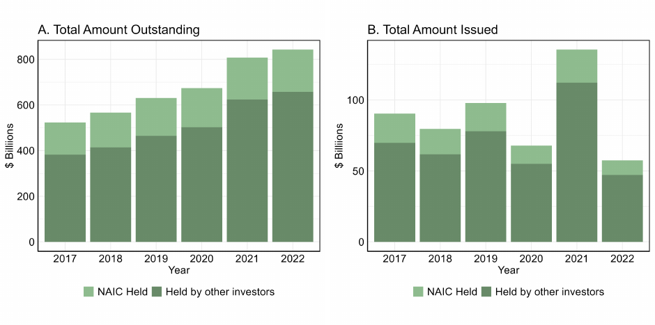
Figure 5: Insurance Holdings of CMBS

Notes: This ﬁgure shows the total amount outstanding (Panel A) and amount originated (Panel B) of

private-label CMBS per year, diﬀerentiating between the amount held by insurance companies and

that held by other investors. We identify holdings of insurance companies using NAIC Schedule D,

Part 1. Insurer-held amounts are calculated as the sum of the BACV of the CMBS held by insurers.

Amount held by other investors is the residual value relative to the total original balance outstand-

ing/originated in a given year. Both plots exclude interest-only and agency CMBS. Source: Trepp,

NAIC, and authors’ calculations.

Figure 6: % CMBS Portfolio without Oﬃce Exposure

Notes: This ﬁgure shows the share of insurance companies’ private-label CMBS portfolio not ex-

posed to any CRE mortgages linked to properties classiﬁed as Oﬃce. Shares are calculated aggregat-

ing BACV for exposed and non-exposed CMBS, where exposure is deﬁned as any percentage of the

pool of mortgages used to ﬁnance oﬃce CRE. Source: Trepp, NAIC, and authors’ calculations.

Figure 7: CMBS Bonds Held by Insurance Companies—Exposure to Oﬃces

Notes: This ﬁgure shows the distribution of oﬃce-exposed shares of insurance companies’ private-

label CMBS portfolio. The left panel shows the distribution for any oﬃce exposure, and the right

panel shows the distribution conditional on any mortgages having main leases expiring between

2023-2026. Source: Trepp, NAIC, and authors’ calculations.

Figure 8: Distribution of Oﬃce Exposure—CMBS Acquired Before and After COVID-19

Notes: This ﬁgure shows the distribution of oﬃce exposures of CMBS acquired by insurance com-

panies, before and after COVID-19. Percent exposure equals the amount of the pool of mortgages

linked to oﬃce CRE. The left panel plots the distribution of oﬃce exposure for CMBS acquired

between 2017-2019. The right panel plots the distribution of oﬃce exposure for CMBS acquired be-

tween 2020-2022. The width of each distribution bar equals 2%. Source: Trepp, NAIC, and authors’

calculations.

Figure 9: Distribution of Oﬃce Exposure with Leases Expiring—CMBS Acquired Before and

After COVID-19

Notes: This ﬁgure shows the distribution of oﬃce exposures with leases expiring within a certain

time window of CMBS acquired by insurance companies, before and after COVID-19. Percent expo-

sure equals the amount of the pool of mortgages linked to oﬃce CRE whose main lease agreement

expires within that time window. Each panel plots the distribution of security exposures of CMBS

acquired before and after COVID-19, for each time window. Source: Trepp, NAIC, and authors’

calculations.

Figure 10: Bank Holdings of Private-label CMBS

Notes: This ﬁgure shows the total amount of private-label CMBS holdings

of U.S. banks, including held-to-maturity and available-for-sale assets. Top 4

banks are J.P. Morgan Chase, Bank of America, Citigroup, and Wells Fargo.

Large banks are institutions with total assets above $ 100 billion, medium

banks are institutions with total assets between $10 billion and $100 billion,

and small banks are institutions with total assets under $10 billion. We also

exclude TD Bank from the plots as it shows discontinuity in holdings of pri-

vate CMBS in 2018 that is not present on the aggregate series. Source: Call

Reports and authors’ calculations.

Figure 11: Small Banks’ Exposure to Private-Label CMBS

Notes: This ﬁgure shows the number of small U.S. banks which hold private-label CMBS (Panel

A) and the median % share of private-label CMBS out of total assets for small banks with CMBS

exposure (Panel B). Small banks are deﬁned as institutions with total assets under $10 billion.

Source: Call Reports and authors’ calculations.

TABLES

Table 1: Summary Statistics

Panel A. All Properties Mean Median Min Max N

Outstanding Balance 12,126,498.41 4,665,665.69 535.94 9,016,115,069.00 7,081,912

Floating Interest Rate 0.12 0.00 0.00 1.00 7,081,912

Delinquency (90 days) 0.01 0.00 0.00 1.00 7,081,912

Recourse Loan 0.01 0.00 0.00 1.00 7,081,912

Loan Term 228.39 120 1 515 7,010,744

Lease Expiration Year 2026 2024 2016 2099 747,189

Largest Tenant % Sqr Ft 45.11 33.44 0.00 100.00 748,523

Panel B. Oﬃce Mean Median Min Max N

Outstanding Balance 35,592,214.49 17,545,061.17 6,760.18 3,000,000,000.00 276,561

Floating Interest Rate 0.08 0.00 0.00 1.00 276,561

Delinquency (90 days) 0.01 0.00 0.00 1.00 276,561

Recourse Loan 0.02 0.00 0.00 1.00 276,561

Loan Term 112.87 120 1 363 275,307

Lease Expiration Year 2025 2024 2016 2099 209,965

Largest Tenant % Sqr Ft 42.20 29.71 0.00 100.00 211,306

Panel C. Retail Mean Median Min Max N

Outstanding Balance 17,123,979.19 7,331,549.50 797.55 2,400,000,000.00 516,328

Floating Interest Rate 0.02 0.00 0.00 1.00 516,328

Delinquency (90 days) 0.02 0.00 0.00 1.00 516,328

Recourse Loan 0.01 0.00 0.00 1.00 516,328

Loan Term 123.63 120 1 360 506,734

Lease Expiration Year 2027 2024 2016 2099 415,663

Largest Tenant % Sqr Ft 45.68 34.52 0.00 100.00 417,838

Notes: This table shows summary statistics from our sample of commercial real estate mortgages. The sample

period is from Jan/2017 to Jun/2022. Panel A includes summary statistics for all property types in the sample.

Panel B includes summary statistics for properties classiﬁed as Oﬃce. Panel C includes summary statistics for

properties classiﬁed as Retail. Source: Trepp and authors’ calculations.

Table 2: Triple Diﬀerences—Lease Expiration Before and After COVID-19

D90

jrt

(1) (2) (3)

P ost Expiration

0.0131

∗∗∗

0.0132

∗∗∗

0.0140

∗∗∗

(0.0029) (0.0029) (0.0034)

P ost Covid

× P ost Expiration

-0.0029 -0.0029 -0.0013

(0.0033) (0.0033) (0.0040)

P ost Covid

× Ind Of f ice

-0.0162

∗∗∗

-0.0160

∗∗∗

-0.0216

∗∗∗

(0.0019) (0.0019) (0.0031)

P ost Expiration

× Ind Of f ice

0.0013 0.0014 0.0004

(0.0062) (0.0062) (0.0068)

P ost Covid

× P ost Expiration

× Ind Of f ice

0.0122

∗

0.0121

∗

0.0132

∗

(0.0064) (0.0064) (0.0074)

Observations 751,294 751,294 751,294

0.42319 0.42324 0.57382

Within R

0.00208 0.00206 0.00300

Month-year ﬁxed eﬀects ✓

Loan ID ﬁxed eﬀects ✓ ✓ ✓

Month-year × Floating ﬁxed eﬀects ✓ ✓

Month-year × City ﬁxed eﬀects ✓

Notes: This table shows the eﬀects of lease expiration on delinquency rates for mortgages

linked to diﬀerent property types, before and after COVID-19, as in (2). The level of obser-

vation is loan j in city r in month t, where month denotes the distribution month of each

securitized mortgage. The sample period is Jan/2017 to Jun/2022. The dependent variable

D90

jrt

is a dummy variable which equals 1 if a loan is at least 90 days past due. P ost Covid

equals 1 after March 2020, P ost Expiration

equals 1 if loan j had its main lease expiration

before or in month t, and Ind Of f ice

equals 1 if loan j is linked to an oﬃce. Standard errors

clustered at the loan level in parentheses. Sources: Trepp and authors’ calculations.

Table 3: Triple Diﬀerences and Occupancy %—Lease Expiration Before and After COVID-19

D90

jrt

(1) (2) (3) (4) (5) (6) (7) (8) (9)

P ost Expiration

0.0185 0.0185 -0.0038 0.0129

∗∗∗

0.0130

∗∗∗

0.0128

∗∗∗

0.0119

∗∗∗

0.0120

∗∗∗

0.0118

∗∗∗

(0.0175) (0.0176) (0.0340) (0.0029) (0.0029) (0.0036) (0.0030) (0.0030) (0.0037)

P ost Covid

× P ost Expiration

0.0535

∗

0.0535

∗

0.0809 -0.0059

∗

-0.0059

∗

-0.0055 -0.0050 -0.0051 -0.0041

(0.0294) (0.0295) (0.0638) (0.0034) (0.0034) (0.0041) (0.0034) (0.0034) (0.0041)

P ost Covid

× Ind Of f ice

-0.0156

∗∗∗

-0.0156

∗∗∗

-0.0264

∗∗

-0.0155

∗∗∗

-0.0154

∗∗∗

-0.0210

∗∗∗

-0.0157

∗∗∗

-0.0155

∗∗∗

-0.0223

∗∗∗

(0.0030) (0.0030) (0.0113) (0.0025) (0.0025) (0.0042) (0.0025) (0.0025) (0.0040)

P ost Expiration

× Ind Of f ice

0.0488 0.0490 0.0720 -0.0046 -0.0046 -0.0056 -0.0035 -0.0034 -0.0044

(0.0366) (0.0367) (0.0558) (0.0064) (0.0064) (0.0070) (0.0064) (0.0064) (0.0071)

P ost Covid

× P ost Expiration

× Ind Of f ice

-0.0725

∗∗

-0.0727

∗∗

-0.1139 0.0169

∗∗

0.0168

∗∗

0.0207

∗∗

0.0162

∗∗

0.0161

∗∗

0.0205

∗∗

(0.0363) (0.0363) (0.0721) (0.0071) (0.0071) (0.0082) (0.0071) (0.0071) (0.0082)

Full

-0.0058 -0.0057 -0.0036

(0.0119) (0.0119) (0.0163)

P ost Covid

× Full

-0.0084

∗∗

-0.0084

∗∗

-0.0035

(0.0034) (0.0034) (0.0056)

P ost Expiration

× Full

0.0131 0.0131 0.0079

(0.0146) (0.0146) (0.0158)

Ind Of f ice

× Full

-0.0016 -0.0015 -0.0093

(0.0131) (0.0131) (0.0180)

P ost Covid

× P ost Expiration

× Full

0.0544

∗

0.0544

∗

0.0626

(0.0298) (0.0298) (0.0406)

P ost Covid

× Ind Of f ice

× Full

−8.32 × 10

−6

-0.0002 0.0038

(0.0039) (0.0040) (0.0066)

P ost Expiration

× Ind Of f ice

× Full

0.0416 0.0415 0.0538

(0.0325) (0.0325) (0.0364)

P ost Covid

× P ost Expiration

× Ind Of f ice

× Full

-0.0838

∗∗

-0.0839

∗∗

-0.1170

∗∗

(0.0360) (0.0360) (0.0465)

Observations 135,346 135,346 135,346 611,679 611,679 611,679 747,025 747,025 747,025

0.44563 0.44565 0.71391 0.43901 0.43908 0.60674 0.43801 0.43807 0.58513

Within R

0.01021 0.01021 0.01239 0.00153 0.00150 0.00233 0.00283 0.00282 0.00373

Month-year ﬁxed eﬀects ✓ ✓ ✓

Loan ID ﬁxed eﬀects ✓ ✓ ✓ ✓ ✓ ✓ ✓ ✓ ✓

Month-year × Floating ﬁxed eﬀects ✓ ✓ ✓ ✓ ✓ ✓

Month-year × City ﬁxed eﬀects ✓ ✓ ✓

Notes: This table shows the eﬀects of lease expiration on delinquency rates of mortgages linked to diﬀerent property types, before and after COVID-19, for partial and full tenant

occupancy. We estimate (2) for the sample of full (columns (1)-(3)) and partial (columns (4)-(6)) occupancy mortgages, and for the whole sample, adding an interaction with the

Full

dummy (columns (7)-(9)). The level of observation is loan j in city r in month t, where month denotes the distribution month of each securitized mortgage. The sample

period is Jan/2017 to Jun/2022. The dependent variable I

D90

jrt

is a dummy variable which equals 1 if a loan is at least 90 days past due. P ost Covid

equals 1 after March 2020,

P ost Expiration

equals 1 if loan j had its main lease expiration before or in month t, Ind Of f ice

equals 1 if loan j is linked to an oﬃce, and Full

is a dummy which equals 1 for

full tenant occupancy. Standard errors clustered at the loan level in parentheses. Sources: Trepp and authors’ calculations.

Table 4: CMBS Bond Trading—Underlying Lease Expiration and Mortgage Delinquency

sold

ijt

(1) (2) (3) (4)

Exp

0.0029 0.0017

(0.0029) (0.0031)

Exp Of f ice

0.0023

(0.0021)

0.0086

∗∗∗

0.0086

∗∗∗

(0.0027) (0.0028)

D Of f ice

0.0093

∗∗

(0.0046)

Observations 176,824 176,824 176,824 176,176

0.63398 0.63399 0.63403 0.63366

Within R

1.7 × 10

−5

3.27 × 10

−5

0.00016 0.00025

Year × Insurer ID ﬁxed eﬀects ✓ ✓ ✓ ✓

CUSIP × Insurer ID ﬁxed eﬀects ✓ ✓ ✓ ✓

Year × Coupon Type ﬁxed eﬀects ✓ ✓ ✓ ✓

Year × NAIC Designation ﬁxed eﬀects ✓ ✓ ✓ ✓

Notes: This table shows the eﬀect of exposure to underlying lease expiration and delinquent

loans (for all properties and for oﬃces) on the likelihood of sales of private-label CMBS by

insurance companies, as in (3). The level of observation is bond j held by insurer i at the

end of year t. The sample period is 2017 to 2022. The dependent variable I

sold

ijt

is a dummy

which equals 1 if bond j was sold by insurer i in year t. I

and I

Y Of f ice

(with Y ∈ {Exp,D})

are dummies equal to 1 if bond j is exposed to mortgages whose main lease expires up until

one year ahead (Exp) or have underlying delinquent mortgages (D), for all properties and only

oﬃces, respectively. Coupon Type is the type of coupon payment for bond j (e.g. ﬁxed rate,

ﬂoating rate, interest only). Standard errors clustered at the security level in parentheses.

Sources: Trepp, NAIC, and authors’ calculations.

Table 5: CMBS Trading Diﬀerence-in-Diﬀerences—Exposure to Lease Expiration

sold

ijt

Lease expiration horizon (τ = 1) (τ = 2) (τ = 3) (τ = 4) (τ = 5) (τ = 6)

Exp(τ)

0.0015 0.0006 0.0033 -0.0008 0.0034 0.0038

(0.0033) (0.0045) (0.0052) (0.0059) (0.0069) (0.0072)

Exp Of f ice(τ)

0.0019 0.0029 0.0040 0.0054 0.0023 0.0026

(0.0028) (0.0031) (0.0037) (0.0045) (0.0058) (0.0066)

Of f ice

-0.0171 -0.0126 -0.0115 -0.0130 -0.0139 -0.0152

(0.0207) (0.0209) (0.0209) (0.0209) (0.0207) (0.0207)

P ost Covid

× I

Exp(τ)

0.0012 0.0101

∗

0.0166

∗∗

0.0071 0.0019 -0.0066

(0.0048) (0.0060) (0.0070) (0.0075) (0.0085) (0.0089)

P ost Covid

× I

Exp Of f ice(τ)

-0.0009 0.0062 0.0068 0.0128

∗∗

0.0181

∗∗

0.0254

∗∗∗

(0.0037) (0.0043) (0.0053) (0.0061) (0.0079) (0.0087)

P ost Covid

× I

Of f ice

0.0237

∗∗∗

0.0140

∗

0.0094 0.0107 0.0097 0.0084

(0.0070) (0.0074) (0.0075) (0.0075) (0.0077) (0.0078)

Observations 219,731 219,731 219,731 219,731 219,731 219,731

0.60744 0.60754 0.60762 0.60757 0.60755 0.60757

Within R

0.00024 0.00049 0.00069 0.00057 0.00053 0.00058

Year × Insurer ID ﬁxed eﬀects ✓ ✓ ✓ ✓ ✓ ✓

CUSIP × Insurer ID ﬁxed eﬀects ✓ ✓ ✓ ✓ ✓ ✓

Year × Coupon Type ﬁxed eﬀects ✓ ✓ ✓ ✓ ✓ ✓

Year × NAIC Designation ﬁxed eﬀects ✓ ✓ ✓ ✓ ✓ ✓

Notes: This table shows the eﬀect of exposure to underlying lease expiration and oﬃces on the likelihood of

sales of private-label CMBS by insurance companies, as in (4). The level of observation is bond j held by insurer

i at the end of year t. The sample period is 2017 to 2022. The dependent variable I

sold

ijt

is a dummy which equals

1 if bond j was sold by insurer i in year t. P ost Covid

equals 1 after 2019, I

Exp(τ)

and I

Exp Of f ice(τ)

are dummies

which equal 1 if bond j is exposed to mortgages whose main lease expires up until year t + τ (excluding year t),

for all properties and only oﬃces, respectively. I

Of f ice

is a dummy which equals 1 for any exposure to oﬃces.

Coupon Type is the type of coupon payment for bond j (e.g. ﬁxed rate, ﬂoating rate, interest only). Standard

errors clustered at the security level in parentheses. Sources: Trepp, NAIC, and authors’ calculations.

Table 6: CMBS Trading Diﬀerence-in-Diﬀerences—Exposure to Lease Expiration of Oﬃces

vs. Other Properties

sold

ijt

Lease expiration horizon (τ = 1) (τ = 2) (τ = 3) (τ = 4) (τ = 5) (τ = 6)

Exp Of f ice(τ)

0.0034 0.0035 0.0031 0.0036 0.0021 0.0020

(0.0025) (0.0028) (0.0033) (0.0040) (0.0049) (0.0054)

Exp Retail(τ)

0.0030 0.0012 0.0042 0.0043 0.0059 0.0067

(0.0025) (0.0033) (0.0043) (0.0053) (0.0064) (0.0066)

Exp Other(τ)

0.0003 0.0044 0.0104

∗∗∗

0.0076

∗∗

0.0072

∗

0.0074

(0.0027) (0.0028) (0.0032) (0.0036) (0.0040) (0.0047)

Retail

-0.0269 -0.0246 -0.0247 -0.0242 -0.0217 -0.0242

(0.0316) (0.0315) (0.0314) (0.0313) (0.0312) (0.0311)

Of f ice

-0.0096 -0.0090 -0.0088 -0.0086 -0.0081 -0.0086

(0.0213) (0.0213) (0.0212) (0.0211) (0.0211) (0.0212)

P ost Covid

× I

Exp Of f ice(τ)

-0.0028 0.0061 0.0099

∗∗

0.0101

∗

0.0074 0.0123

∗

(0.0033) (0.0039) (0.0047) (0.0054) (0.0065) (0.0072)

P ost Covid

× I

Exp Retail(τ)

-0.0048 0.0019 0.0072 0.0072 0.0161

∗

0.0047

(0.0035) (0.0048) (0.0068) (0.0076) (0.0090) (0.0094)

P ost Covid

× I

Exp Other(τ)

0.0007 -0.0057

∗

-0.0078

∗∗

-0.0031 -0.0005 0.0022

(0.0036) (0.0034) (0.0038) (0.0043) (0.0047) (0.0050)

P ost Covid

× I

Retail

0.0291

∗∗∗

0.0242

∗∗∗

0.0193

∗∗

0.0171

∗∗

0.0101 0.0155

∗

(0.0064) (0.0069) (0.0077) (0.0080) (0.0083) (0.0086)

P ost Covid

× I

Of f ice

0.0201

∗∗∗

0.0157

∗∗

0.0121 0.0104 0.0082 0.0075

(0.0069) (0.0071) (0.0074) (0.0075) (0.0077) (0.0079)

Observations 219,731 219,731 219,731 219,731 219,731 219,731

0.60756 0.60761 0.60771 0.60767 0.60769 0.60768

Within R

0.00054 0.00068 0.00092 0.00083 0.00089 0.00086

Year × Insurer ID ﬁxed eﬀects ✓ ✓ ✓ ✓ ✓ ✓

CUSIP × Insurer ID ﬁxed eﬀects ✓ ✓ ✓ ✓ ✓ ✓

Year × Coupon Type ﬁxed eﬀects ✓ ✓ ✓ ✓ ✓ ✓

Year × NAIC Designation ﬁxed eﬀects ✓ ✓ ✓ ✓ ✓ ✓

Notes: This table shows the eﬀect of exposure to underlying lease expiration and oﬃces on the likelihood of

sales of private CMBS by insurance companies, as in (6). The level of observation is bond j held by insurer i at

the end of year t. The sample period is 2017 to 2022. The dependent variable I

sold

ijt

is a dummy which equals

1 if bond j was sold by insurer i in year t. P ost Covid

equals 1 after 2019 and I

Exp Retail(τ)

, I

Exp Of f ice(τ)

and

Exp Other(τ)

are dummies which equal 1 if bond j is exposed to mortgages whose main lease expires up until

year t + τ (excluding year t), for retail, oﬃces, and other properties, respectively. I

Retail

and I

Of f ice

equal 1 for

any exposure to retail and oﬃces, respectively. Coupon Type is the type of coupon payment for bond j (e.g.

ﬁxed rate, ﬂoating rate, interest only). Standard errors clustered at the security level in parentheses. Sources:

Trepp, NAIC, and authors’ calculations.

Table 7: Bond Pricing

Coupon

(1) (2) (3) (4)

Of f ice

% -0.0043

∗∗∗

-0.0115

∗∗∗

-0.0117

∗∗∗

-0.0068

∗∗

(0.0016) (0.0037) (0.0040) (0.0035)

Of f ice

% × P ost Covid

-0.0015 -0.0124

∗∗

-0.0113

∗∗

-0.0136

∗∗∗

(0.0023) (0.0051) (0.0051) (0.0050)

Of f ice

% × NAIC Held

0.0099

∗∗∗

0.0085

∗∗

0.0042

(0.0036) (0.0036) (0.0032)

Of f ice

% × P ost Covid

× NAIC Held

0.0147

∗∗∗

0.0148

∗∗∗

0.0175

∗∗∗

(0.0049) (0.0047) (0.0045)

Retail

% -0.0109

∗∗

(0.0053)

P ost Covid

× Retail

% -0.0005

(0.0076)

Retail

% × NAIC Held

0.0115

∗∗

(0.0051)

Retail

% × P ost Covid

× NAIC Held

0.0137

∗

(0.0077)

P rime rating

-0.6106

∗∗∗

-0.0996

∗

(0.0404) (0.0546)

Main state (share in %)

0.0003 0.0077

∗∗∗

(0.0015) (0.0020)

Num Loans at Securitization

-0.0062

∗∗∗

-0.0065

∗∗∗

(0.0017) (0.0018)

Horizontal Risk Retention

0.0495 0.0076

(0.0369) (0.0407)

W eighted Avg LT V at Securitization

0.0396

∗∗∗

(0.0078)

W eighted Avg DSCR at Securitization

0.1950

∗∗

(0.0850)

Conduit

-0.3504

∗∗

(0.1367)

Observations 3,302 3,302 3,302 2,529

0.58652 0.61258 0.64864 0.67202

Within R

0.02036 0.08209 0.15321 0.23219

Year-quarter × Maturity ﬁxed eﬀects ✓ ✓ ✓ ✓

Lead Underwriter ﬁxed eﬀects ✓ ✓

Notes: This table shows a regression of ﬁxed rate bond coupons of private-label CMBS on the oﬃce collateral

and insurance ownership before and after COVID-19, as in (7). The level of observation is bond j originated

in quarter t. The sample period is 2017 to 2022. The dependent variable Coupon

is the coupon rate of

ﬁxed rate bond j originated in quarter t. P ost Covid

equals 1 after 2019. NAIC Held

equals 1 if bond j is

held by any insurer in the end of the year of origination of the respective quarter t. Of f ice

% and Retail

% are the percent shares of the deal linked to oﬃce and retail loans. P rime rating

equals 1 if the bond is

rated at least BBB by S&P or by Fitch or at least Baa3 by Moody’s. Main State (share in %)

is the share

of the deal invested in the main state. N um of Loans at Securitization

is the number of loans in the deal

at origination. Horizontal Risk Retention

and Conduit

are dummies for deals of each type, respectively.

W eighted Avg LT V at Securitization

and W eighted Avg DSCR at Securitization

are average LTV and DSCR

weighted by loan volume within each deal. Standard errors clustered at the security level in parentheses.

Sources: Trepp, NAIC, and authors’ calculations.

Table 8: Insurer CMBS Portfolio Exposure and Asset Sales

sold

ijt

Risky

Downgrade

jt−1

(1) (2) (3) (4) (5) (6)

× T

Of f ice

it−1

-0.0008 -0.0016 -0.0017 0.0015 0.0102

∗∗∗

0.0103

∗∗∗

(0.0021) (0.0035) (0.0035) (0.0021) (0.0040) (0.0039)

× T

Retail

it−1

0.0007 0.0006 -0.0070

∗∗

-0.0071

∗∗

(0.0024) (0.0024) (0.0029) (0.0029)

× T

Lodging

it−1

0.0023 0.0040 -0.0051 -0.0057

(0.0071) (0.0070) (0.0067) (0.0068)

P ost Covid

× I

× T

Of f ice

it−1

-0.0022 -0.0095

∗∗∗

-0.0093

∗∗∗

-0.0007 -0.0117

∗∗

-0.0117

∗∗

(0.0021) (0.0035) (0.0034) (0.0027) (0.0046) (0.0046)

P ost Covid

× I

× T

Retail

it−1

0.0078

∗∗

0.0076

∗∗

0.0094

∗∗

0.0095

∗∗

(0.0031) (0.0031) (0.0038) (0.0037)

P ost Covid

× I

× T

Lodging

it−1

0.0056 0.0042 0.0069 0.0085

(0.0069) (0.0069) (0.0094) (0.0093)

× T

%CorpBonds

it−1

0.0401

∗∗∗

-0.0076

(0.0137) (0.0115)

P ost Covid

× I

× T

%CorpBonds

it−1

-0.0282

∗

0.0241

(0.0146) (0.0150)

Observations 7,091,153 7,091,153 7,091,153 5,605,453 5,605,453 5,605,453

0.71081 0.71082 0.71083 0.78171 0.78171 0.78171

Within R

0.00086 0.00090 0.00093 6.25 × 10

−6

1.55 × 10

−5

1.95 × 10

−5

Year × CUSIP ﬁxed eﬀects ✓ ✓ ✓ ✓ ✓ ✓

CUSIP × Insurer ID ﬁxed eﬀects ✓ ✓ ✓ ✓ ✓ ✓

Year × Insurer ID ﬁxed eﬀects ✓ ✓ ✓ ✓ ✓ ✓

Notes: This table shows the eﬀect of exposure to diﬀerent types of collateral via CMBS holdings on the likelihood of

sales of risky assets by insurance companies, as in (8). The level of observation is bond j originated in quarter t. The

sample period is 2017 to 2022, and the sample includes all bonds. The dependent variable I

sold

ijt

is a dummy which

equals 1 if bond j was sold by insurer i in year t. P ost Covid

equals 1 after 2019, T

P rop

it−1

is the size of the exposure

of insurance company i to property type P rop ∈ {Of f ice, Retail, Lodging} in year t − 1, and I

is a dummy which

equals 1 if the bond is classiﬁed as Risky or if it was downgraded in year t − 1. T

%CorpBonds

it−1

is the share of insurance

company i ﬁxed income portfolio invested in corporate bonds in year t − 1. Standard errors clustered at the insurer

level in parentheses. Sources: Trepp, NAIC, and authors’ calculations.

Table 9: CMBS Bank Buyer Diﬀerence-in-Diﬀerences—Exposure to Lease Expiration

sold to bank

ijt

Lease expiration horizon (τ = 1) (τ = 2) (τ = 3) (τ = 4) (τ = 5) (τ = 6)

Exp(τ)

0.0023

∗

0.0046

∗∗∗

0.0057

∗∗∗

0.0068

∗∗∗

0.0061

∗∗∗

0.0055

∗∗

(0.0012) (0.0017) (0.0019) (0.0021) (0.0023) (0.0022)

Exp Of f ice(τ)

0.0015 0.0016 0.0020 0.0021 0.0025 0.0035

(0.0011) (0.0012) (0.0015) (0.0019) (0.0022) (0.0021)

Of f ice

-0.0012 -0.0016 -0.0022 -0.0031 -0.0029 -0.0026

(0.0068) (0.0068) (0.0068) (0.0069) (0.0069) (0.0068)

P ost Covid

× I

Exp(τ)

-0.0018 -0.0025 -0.0037 -0.0062

∗∗

-0.0064

∗∗

-0.0057

∗∗

(0.0016) (0.0021) (0.0024) (0.0026) (0.0026) (0.0027)

P ost Covid

× I

Exp Of f ice(τ)

-0.0011 0.0006 0.0020 0.0032 0.0046

∗∗

0.0051

∗∗

(0.0014) (0.0015) (0.0018) (0.0021) (0.0024) (0.0025)

P ost Covid

× I

Of f ice

0.0050

∗∗

0.0047

∗

0.0044 0.0049

∗

0.0037 0.0027

(0.0024) (0.0026) (0.0027) (0.0028) (0.0027) (0.0028)

Observations 203,987 203,987 203,987 203,987 203,987 203,987

0.39349 0.39355 0.39361 0.39363 0.39362 0.39366

Within R

0.00012 0.00022 0.00031 0.00036 0.00034 0.00040

Year × Insurer ID ﬁxed eﬀects ✓ ✓ ✓ ✓ ✓ ✓

CUSIP × Insurer ID ﬁxed eﬀects ✓ ✓ ✓ ✓ ✓ ✓

Year × Coupon Type ﬁxed eﬀects ✓ ✓ ✓ ✓ ✓ ✓

Year × NAIC Designation ﬁxed eﬀects ✓ ✓ ✓ ✓ ✓ ✓

Notes: This table shows the eﬀect of exposure to underlying lease expiration and oﬃces on the likelihood of sales of

private-label CMBS by insurance companies to banks. The level of observation is bond j held by insurer i at the end of

year t. The sample period is 2017 to 2022. The dependent variable I

sold to bank

ijt

is a dummy which equals 1 if bond j was

sold by insurer i in year t to a bank. We excluded CMBS holdings where the following ﬁrms are buyers: FA REINSUR-

ANCE, Resolution Life Insurance, Coinsurance Talcott-Allianz. P ost Covid

equals 1 after 2019, I

Exp(τ)

and I

ExpOf f ice(τ)

are dummies which equal 1 if bond j is exposed to mortgages whose main lease expires up until year t + τ (excluding year

t), for all properties and only oﬃces, respectively. I

Of f ice

is a dummy which equals 1 for any exposure to oﬃces. Standard

errors clustered at the security level in parentheses. Coupon Type is the type of coupon payment for bond j (e.g. ﬁxed

rate, ﬂoating rate, interest only). Sources: Trepp, NAIC, and authors’ calculations.

Appendix

A. Additional Figures and Tables

Figure A.1: Delinquency Rates by Property Type

Notes: This Figure reports average delinquency for mortgages linked to diﬀerent property types.

Property types are deﬁned as in Appendix B. Delinquency is a dummy variable which equals 1 if a

mortgage is more than 90 days past due. Source: Trepp and authors’ calculations.

A-1

Figure A.2: Distribution of % Occupancy by Largest Tenant

Notes: This ﬁgure shows the distribution of the % occupied by the largest tenant in the properties

linked to CRE mortgages, separately for Retail and Oﬃce. The width of each distribution bar is 4%.

Source: Trepp and authors’ calculations.

A-2

Figure A.3: Distribution of % Teleworkable Jobs—All MSAs and Oﬃce Mortgages

Notes: This ﬁgure shows the distribution of the share of jobs in each MSA that can be performed

from home, using the measure proposed by Dingel and Neiman (2020). We plot the distribution of

all MSAs in the Dingel and Neiman (2020) dataset, and the distribution of the MSAs from the mort-

gages in the Trepp data, focusing on properties classiﬁed as Oﬃce. The width of each distribution

bar is 2%. Source: Trepp and authors’ calculations.

A-3

Figure A.4: Dynamic Diﬀerence-in-Diﬀerences: Trading of CMBS Exposed to Cash Flow

Risks

Notes: Each plot shows the dynamic eﬀect of exposure to underlying oﬃce lease expiration on the likelihood of

sales of private-label CMBS by insurers, as in speciﬁcation (5). The level of observation is bond j held by insurer

i at the end of year t. The dependent variable I

sold

ijt

is a dummy which equals 1 if bond j was sold by insurer i

in year t. The sample period is 2017 to 2022. I

ExpOf f ice(τ)

is deﬁned as in the main paper, and D

ExpOf f ice(τ)

are

dummies equal to 1 if bond j is exposed to mortgages whose main lease expires up until one year ahead and

ι = t. Source: Trepp, NAIC, and authors’ calculations.

A-4

Figure A.5: Share Insurers CMBS Portfolio Exposed to Lease Expiration Within τ years

Notes: Each plot shows the share of the private-label CMBS portfolio of insurance companies at the

end of each year, for bonds which have I

ExpOf f ice(τ)

equal 1, that is, bond j has any underlying oﬃce-

linked mortgages whose leases expire within τ years in year t. Source: Trepp, NAIC, and authors’

calculations.

A-5

Figure A.6: Buyers of CMBS by Category over Time (All Properties)

Notes: This ﬁgure reports the share of buyers of all private-

label CMBS against all properties sold by insurance ﬁrms by cat-

egories over time. We exclude three major buyers (FA REIN-

SURANCE, RESOLUTION LIFE, COINSURANCE TALCOTT-

ALLIANZ). Property types are deﬁned as in Appendix B. Source:

Trepp, NAIC, and authors’ calculations.

A-6

Figure A.7: Buyers of CMBS by Category over Time (Oﬃces)

Notes: This ﬁgure reports the share of buyers of all private-label

CMBS against oﬃces sold by insurance ﬁrms by categories over

time. We exclude three major buyers (FA REINSURANCE, RES-

OLUTION LIFE, COINSURANCE TALCOTT-ALLIANZ). Property

types are deﬁned as in Appendix B. Source: Trepp, NAIC, and au-

thors’ calculations.

A-7

Table A.1: Property Types and Lease Expiration Information

Property Category # without lease expiration # with lease expiration % with lease expiration

Healthcare-Nursing 464727 51 0.01

Industrial-WH 147055 53515 26.68

Lodging-Restaurants 208574 180 0.09

Mixed Use 66103 56571 46.11

Multifamily 5057710 831 0.02

Oﬃce 66596 209965 75.92

Other 223293 10413 4.46

Retail 100665 415663 80.50

Notes: This table shows the number of observations in our CRE mortgage sample for which the lease expiration informa-

tion is included, and the number of observations for which the lease expiration information is missing. Sample is from

Jan/2017 to Jun/2022. Breakdown is provided by property type. Source: Trepp and authors’ calculations.

A-8

Table A.2: CMBS Insurance Buyer Diﬀerence-in-Diﬀerences—Exposure to Lease Expiration

sold to insurance

ijt

Lease expiration horizon (τ = 1) (τ = 2) (τ = 3) (τ = 4) (τ = 5) (τ = 6)

Exp(τ)

0.0002 0.0009

∗

8.62 × 10

−5

0.0002 8.82 × 10

−5

0.0004

(0.0004) (0.0005) (0.0006) (0.0006) (0.0006) (0.0007)

Exp Of f ice(τ)

0.0003 −4.85 × 10

−5

0.0008 0.0004 0.0007 0.0005

(0.0004) (0.0005) (0.0005) (0.0005) (0.0005) (0.0006)

Of f ice

-0.0017 -0.0015 -0.0017 -0.0017 -0.0018 -0.0019

(0.0013) (0.0013) (0.0013) (0.0013) (0.0013) (0.0013)

P ost Covid

× I

Exp(τ)

−8.79 × 10

−5

0.0004 0.0004 -0.0004 -0.0005 -0.0013

(0.0006) (0.0008) (0.0007) (0.0007) (0.0008) (0.0009)

P ost Covid

× I

Exp Of f ice(τ)

1.5 × 10

−5

8.1 × 10

−5

-0.0002 0.0007 0.0008 0.0018

∗∗

(0.0006) (0.0006) (0.0005) (0.0006) (0.0006) (0.0009)

P ost Covid

× I

Of f ice

-0.0004 -0.0007 -0.0006 -0.0008 -0.0009 -0.0011

(0.0008) (0.0008) (0.0008) (0.0008) (0.0009) (0.0009)

Observations 203,987 203,987 203,987 203,987 203,987 203,987

0.41865 0.41866 0.41866 0.41866 0.41866 0.41868

Within R

2.41 × 10

−5

5.25 × 10

−5

5.34 × 10

−5

4.11 × 10

−5

5.18 × 10

−5

8.35 × 10

−5

Year × Insurer id ﬁxed eﬀects ✓ ✓ ✓ ✓ ✓ ✓

CUSIP × Insurer id ﬁxed eﬀects ✓ ✓ ✓ ✓ ✓ ✓

Year × Coupon Type ﬁxed eﬀects ✓ ✓ ✓ ✓ ✓ ✓

Year × NAIC Designation ﬁxed eﬀects ✓ ✓ ✓ ✓ ✓ ✓

Notes: This table shows the eﬀect of exposure to underlying lease expiration and oﬃces on the likelihood of sales of private-label CMBS by insurance companies

to insurance companies. The level of observation is bond j held by insurer i at the end of year t. The sample period is 2017 to 2022. The dependent variable

sold to insurance

ijt

is a dummy which equals 1 if bond j was sold by insurer i in year t to another insurance company. We excluded CMBS holdings where the following

ﬁrms are buyers: FA REINSURANCE, Resolution Life Insurance, Coinsurance Talcott-Allianz. P ost Covid

equals 1 after 2019, I

Exp(τ)

and I

ExpOf f ice(τ)

are dummies

which equal 1 if bond j is exposed to mortgages whose main lease expires up until year t + τ (excluding year t), for all properties and only oﬃces, respectively. I

Of f ice

is a dummy which equals 1 for any exposure to oﬃces. Coupon Type is the type of coupon payment for bond j (e.g. ﬁxed rate, ﬂoating rate, interest only). Standard

errors clustered at the security level in parentheses. Sources: Trepp, NAIC, and authors’ calculations.

A-9

Table A.3: Small Bank Characteristics by CMBS Ownership

CMBS Before COVID-19 CMBS Only After COVID-19 No CMBS

Total Assets (000s) 1,751,887 1,267,447 707,091

% Non-owner occ CRE loans 16.35 17.16 13.28

% Private CMBS over total assets 1.18 1.26 0

% Private CMBS 1.98 2.37 0

% Short term securities 2.93 2.76 5.55

% US Treasury 8.22 9.56 16.39

% State and Municipal Bonds 28.64 28.67 27.51

% Other Debt Securities 3.28 3.42 1.95

% Foreign Debt Securities 0.13 0.10 0.09

% Agency MBS 10.43 9.83 7.53

Tier 1 Leverage 10.85 10.81 11.57

Notes: This table shows average values for selected characteristics for three types of small banks over the four

quarters of 2023. The ﬁrst column includes all banks that hold private-label CMBS between 2017 and March 2020.

The second column includes all banks that hold private-label CMBS only after March 2020. The last column includes

all remaining banks, i.e., banks that do not hold any private-label CMBS between 2017 and 2023. Source: Call

Reports and authors’ calculations.

A-10

B. Data Construction

Our data comes from two main sources, Trepp and NAIC, and are complemented by Call

Reports data for our bank level analysis. In what follows, we document the data cleaning

procedures for each of the two data sources, and show how we obtain measures of exposure

to cash ﬂow shocks at the CMBS level.

Trepp CRE mortgage data. Mortgage data is informed at the loan level with frequency dic-

tated by distribution dates (ddate). We use these distribution dates as our main date variables

in the loan level analysis. In constructing our sample for the analysis, we exclude:

• Observations without city information;

• Observations with an outstanding balance lower than $ 500;

• Observations for which lease expiration is patchy, that is, when lease expiration infor-

mation exists for certain months, ceases to be included, and is again included after-

wards;

• Observations which have more than one broad property type associated with it in the

year in our sample.

Furthermore, we use information from the variable proptype, informed by Trepp, to con-

struct the broad property types which we use in our analysis. The variable proptype has a

large number of stringers indicating the use of the property serving as collateral for each

mortgages. We aggregate these strings into eight diﬀerent property types: Oﬃce, Retail, Mul-

tifamily, Mixed Use, Healthcare-Nursing, Lodging-Restaurants, Industrial and Warehouses, and

the residual category Other. Examples of how we bin diﬀerent proptype into our broader

property type category are:

• Oﬃce includes proptype strings such as “Oﬃce” “Oﬃce/Hdqr”,“Oﬃce Building” and

“oﬃce properties”;

• Retail includes proptype strings such as “Retail”, “Retail Unanchored”, “Retail An-

chored” and “Retail Mall”;

B-1

• Multifamily includes proptype strings such as “Multi-Tenant”, “Multifamily” and “Multi-

family”;

• Mixed Use includes proptype strings such as “Mixed-Use”, “Oﬃce/Warehouse”, “Mul-

tifamily/Retail” and “Oﬀc/Retail/Mltfmly”;

• Healthcare-Nursing includes proptype strings such as “Nursing Home”, “Medical Of-

ﬁce”, “Assisted Living” and “Medical Oﬃce”;

• Lodging-Restaurants includes proptype strings such as “Hospitality”, “Lodging Full

Service”, “Restaurant” and “Hotel”;

• Industrial and Warehouses includes proptype strings such as “Industrial”, “Self-Storage”,

“Warehouse” and “Industrial/warehouse”.

The full list of strings and their respectively classiﬁcation can be obtained upon request.

Following this procedure, we obtain the loan level monthly panel summarized in Table 1.

Call Reports. We obtain bank level data at quarterly frequency from the Reports of Condi-

tion and Income (call reports), available here. We construct our series of holdings of private

CMBS by following the construction of the LM763063653.Q and LM763063693.Q variables

at the bank level. Detailed instructions for the construction of these two series can be found

here and in here.

B.1. CMBS and Insurer Level Exposure to Underlying Loan Characteristics

Since NAIC data is at annual frequency and Trepp data is at distribution date frequency

(monthly), we follow an aggregation procedure to plug loan information into CMBS. Specif-

ically, we collect deal level information corresponding to December of each year (and June

for 2022, the last month in our sample from Trepp), and add this information to the bonds

linked to each deal.

We exclude TD Bank from the analysis as its holdings of private-label CMBS suddenly drop in 2018, and

no discontinuous drop is observed in either of the aggregate series. Our small bank analysis is identical as TD

Bank would not be classiﬁed as a small bank.

B-2

Speciﬁcally, let T otAmt

djt

denote the total amount outstanding of the pool of loans of deal

d which is linked to bond j and T otAmt

Of f ices

djt

denote the same amount for loans linked to of-

ﬁce properties. Then bond j’s exposure to oﬃces in year t is deﬁned as T

Of f ice

≡

T otAmt

Of f ices

djt

T otAmt

djt

This exposure variable is used to construct dummy variables for positive exposure to oﬃces

using variables analogous to T otAmt

Of f ices

djt

that only include amount for loans with leases

expiring within each τ horizon.

To obtain insurer level exposures, we calculate a weighted average exposure at the bond

level (weighted by BACV), times the size of the portfolio of private-label CMBS for each

insurer.

B-3

C. Identifying Active Sales and Acquisitions

The results in Section 5 rely on measures of active asset sales and acquisitions by insurers,

obtained from NAIC Schedule D, parts 3 and 4. We identify active sales using a procedure

similar to Becker, Opp and Saidi (2022). First, we use the information contained in the

variable name of the purchaser to exclude entries with keywords associated with maturity,

redemption, repayment and default, for example. We also impose the requirement of strict

positive or negative value in the variable realized gain(loss) on disposal. Finally, we further

exclude observations for which maturity dates coincide with the report date.

To classify active acquisitions, we identify a series of keywords for the vendor variable

which contain information not associated with active acquisitions. These keywords include

references to exchange, capitalization, merger and transfer, for example. The full list of key-

words, alongside the R code, can be obtained from the authors upon request.

C-1