
University of New Orleans University of New Orleans
ScholarWorks@UNO ScholarWorks@UNO
University of New Orleans Theses and
Dissertations
Dissertations and Theses
5-2023
Automating Lackenby's Method: The Design of a Set of Scripts to Automating Lackenby's Method: The Design of a Set of Scripts to
Execute Lackenby's Method with McNaull's Expansion in Execute Lackenby's Method with McNaull's Expansion in
Rhinoceros 3D Rhinoceros 3D
Mara E. Kramer
University of New Orleans
Follow this and additional works at: https://scholarworks.uno.edu/td
Part of the Other Engineering Commons
Recommended Citation Recommended Citation
Kramer, Mara E., "Automating Lackenby's Method: The Design of a Set of Scripts to Execute Lackenby's
Method with McNaull's Expansion in Rhinoceros 3D" (2023).
University of New Orleans Theses and
Dissertations
. 3062.
https://scholarworks.uno.edu/td/3062
This Thesis is protected by copyright and/or related rights. It has been brought to you by ScholarWorks@UNO with
permission from the rights-holder(s). You are free to use this Thesis in any way that is permitted by the copyright
and related rights legislation that applies to your use. For other uses you need to obtain permission from the rights-
holder(s) directly, unless additional rights are indicated by a Creative Commons license in the record and/or on the
work itself.
This Thesis has been accepted for inclusion in University of New Orleans Theses and Dissertations by an
authorized administrator of ScholarWorks@UNO. For more information, please contact scholar[email protected].
Automating Lackenby’s Method: The Design of a Set of Scripts to Execute Lackenby’s Method
with McNaull’s Expansion in Rhinoceros 3D
A Thesis
Submitted to the Graduate Faculty of the
University of New Orleans
in partial fulfillment of the
requirements for the degree of
Master of Science in Engineering
in
Engineering
Naval Architecture and Marine Engineering
by
Mara Kramer
B.S. University of New Orleans, 2021
May, 2023
ii
Table of Contents
List of Figures ................................................................................................................................ iii
List of Tables ................................................................................................................................. iv
Abstract ........................................................................................................................................... v
1. Introduction ............................................................................................................................. 1
2. Theory ..................................................................................................................................... 2
2.1. Lackenby’s Method ............................................................................................................ 3
2.2. McNaull’s Modifications .................................................................................................... 6
2.3. Higher Order Moment Derivations ................................................................................... 11
2.4. Akima Interpolation .......................................................................................................... 13
3. Code Overview ..................................................................................................................... 15
3.1. McNaull Cubic Matrix (cubicmatrix.py) .......................................................................... 15
3.2. Sectional Area Calculations (secarea.py) ......................................................................... 16
3.3. Main Script (main.py) ....................................................................................................... 19
4. Introduction to the Sample Vessel ........................................................................................ 26
5. Sample Results and Analysis ................................................................................................ 29
6. Conclusions ........................................................................................................................... 33
References ..................................................................................................................................... 35
Appendix A ................................................................................................................................... 36
Appendix B ................................................................................................................................... 37
Appendix C ................................................................................................................................... 38
Appendix D ................................................................................................................................... 39
Appendix E ................................................................................................................................... 40
Appendix F.................................................................................................................................... 41
Appendix G ................................................................................................................................... 42
Appendix H ................................................................................................................................... 43
Appendix I .................................................................................................................................... 44
Appendix J .................................................................................................................................... 45
Appendix K ................................................................................................................................... 46
Appendix L ................................................................................................................................... 47
Vita ................................................................................................................................................ 48
iii
List of Figures
Figure 1: “One minus prismatic” linear variation of a half-body (Lackenby). ............................... 5
Figure 2: Quadratic variation of a half-body (Lackenby). .............................................................. 6
Figure 3: Cubic variation of a half-body (forebody) (McNaull). .................................................... 7
Figure 4: Discretization of a ship bow into quadrilateral and triangular panels (Birk). ............... 12
Figure 5: Plot of CSV points used to define the four test stations. ............................................... 17
Figure 6: Python generated plot of test sectional areas................................................................. 17
Figure 7: Python generated sectional area curve plot. .................................................................. 19
Figure 8: User interface window that appears when running script. ............................................ 21
Figure 9: Parent hull body plan (top) and half-breadth plan (bottom). ......................................... 26
Figure 10: Parent hull sectional area curve (forebody right). ....................................................... 27
Figure 11: Derived hull lines plan. ............................................................................................... 29
Figure 12: Comparison of parent and derived hull sectional area curves. .................................... 29
Figure 13: Comparison of parent and derived hull body plans. .................................................... 30
iv
List of Tables
Table 1: Half-body variables for “one-minus prismatic” variation (Lackenby). ............................ 4
Table 2: Half-body variables for cubic variation (McNaull). ......................................................... 8
Table 3: Comparison of hand- and Python-calculated areas and centers. .................................... 18
Table 4: Definitions of the variables output from SACfunc. ...................................................... 22
Table 5: Parent hull input values. ................................................................................................. 27
Table 6: Comparison of half-body variables. ............................................................................... 31
v
Abstract
In vessel design, modifying the design of a preexisting hull is a common practice to save
time and labor compared to designing a hull from scratch. This can be achieved either by manually
adjusting the hull model in a 3D modeling software or by systematically adjusting certain vessel
parameters using an algebraic method. However, these methods are time-intensive and do not fully
utilize the capabilities of modern software. To address this issue, this paper presents a set of
Rhinoscript and Python scripts that automate part of the hull modification process using
Lackenby’s method with McNaull’s expansion. The developed code utilizes provided hull offsets
(comma-separated values, CSV, file), along with user-input values, to perform the desired
Lackenby shift. The resulting modified hull surface is displayed in Rhino alongside the original
hull surface. The developed scripts demonstrate the potential of modern software to enhance the
efficiency and accuracy of vessel design.
Keywords: hull design, Lackenby, McNaull, Python, Rhino, Rhinoscript
1
1. Introduction
When designing vessels, modifying existing hull designs to meet current project
specifications is a common tactic for saving labor time and expense. However, many firms do not
take advantage of the capabilities of modern 3D modeling software. Rhinoceros 3D (Rhino) is a
popular software among naval architecture firms, with its own coding language, Rhinoscript, built
off the Python language. While Rhinoscript is admittedly still rather restricted, it can be used to
semi-automate many design processes where a 2D or 3D object is a desired outcome. This project
leverages Rhinoscript to create a set of scripts for modeling a derived hull from a parent hull using
Lackenby’s method with McNaull’s expansion.
This paper presents a breakdown of the operation of each script written, as well as the
theory and methodology for the hull modification methods used within. The main script, written
in Rhinoscript, performs various functions to maximize the program’s potential functionality, with
a focus on reducing user interaction. The script can modify a monohull vessel using user input
values and a comma-separated values (CSV) file containing station offsets, returning 3D surface
models of both the parent and derived hull, as well as data files.
Section 2 delves into the theory behind Lackenby’s method, McNaull’s modifications, and
Akima interpolation – the fundamental theoretical components for this project. Section 3 provides
an overview of each script developed to execute the Lackenby shift in Rhino, discussing their
format and functionality. Section 4 showcases a sample vessel used to demonstrate the code’s
functionality, while Section 5 presents and evaluates the results obtained from the sample vessel.
Finally, Section 6 summarizes the conclusions drawn from this project, discusses future work, and
examines potential applications.
2
2. Theory
Over the years, many methods have been developed to help optimize the hull design
process. One such method, commonly employed in the 1900s, used series of parent hulls as
templates for newly developed hulls. These series documented the best combinations of geometric
variations in length, beam, and depth that resulted in the least amount of resistance for various
vessel forms (planing vessel, tanker, etc.) and were early attempts of systematic variation.
Examples of standard series include: Taylor series, Series 60, Swedish tanker and cargo series,
German HSVA series, and the British BSRA series (Taylor). Interestingly, some standard series
(i.e. the British BSRA series) used Lackenby’s method in development. However, limitations of
this method have become progressively more apparent as vessel designs become increasingly
complex and optimized, particularly in military applications, where the design of vessels is critical
for gaining an edge over potential adversaries.
As a result, new methods (particularly lines distortion and parametric hull generation) have
received increased attention. The dominant methods of lines distortion are Lackenby’s method
(Lackenby) and McNaull’s modification and expansion of Lackenby’s method (McNaull). Two
notable examples of parametric hull design methods are the “Parametric Generation of Yacht
Hulls” (Bole) and “Parametric Design and Hydrodynamic Optimization of Ship Hull Forms”
(Harries). Bole’s report identified factors and parameters critical in yacht design and investigated
several parametric methods to generate a yacht hull form. The parametric methods developed use
a combination of B-splines and defined parameters in order to complete the calculations. While
this method offers a comparative alternative to a lines distortion approach, it is limited in
application to yacht design (Bole).
3
Harries investigates the use of Lackenby’s method for 3D hull modeling and develops a
comprehensive parametric design method intended for use with 3D modeling software and
computer programs. Regarding Lackenby’s method for hull design, Harries concludes that “the
approach is not flexible enough to control the design in detail” and that the method with which
Lackenby’s method is executed is “too inflexible for hydrodynamic improvement in real fluid”.
Harries’s parametric method is particularly suited for 3D software or automation due to its
accuracy in meeting desired properties and ability to maintain fairness of a hull form (Harries).
Theoretically, this parametric method does not have any disadvantages; however, it is not suitable
for use in this project for several reasons:
This method generates a hull form from scratch rather than using a parent hull form
Executing this method is computationally intensive and time-consuming
The current scripting tools available in Rhino are limited and would not be able to
perform the computations required to complete the parametric design method
Therefore, despite its flaws, Lackenby’s method with McNaull’s expansion was chosen for this
project due to its simplicity and suitable accuracy for preliminary hull design.
2.1. Lackenby’s Method
In Lackenby’s 1950 paper “On the Systematic Geometrical Variation of Ship Forms”,
equations for the independent variation of three separate parameters – prismatic coefficient (
),
longitudinal center of buoyancy (LCB), and extent of the parallel midbody ( ) – by distorting the
sectional area curves of a parent vessel were derived. Lackenby’s method was a significant
advancement compared to traditional techniques, such as “swinging” the sectional area curve to
shift the longitudinal center of buoyancy, which lacked control over the position of the parallel
midbody or the positon of the maximum section. McNaull emphasized the importance of

4
Lackenby’s method, stating that it “represented a significant improvement over such traditional
methods” (McNaull).
The first method (“one minus prismatic” variation) presented in Lackenby’s paper splits
the vessel into fore- and aft-bodies at midship so that both ends of the vessel are varied
independently. The term “one minus prismatic” is drawn from the equations derived that share the
term ( ), where is the prismatic coefficient of the half-body. Each half-body uses the same
set of variables as shown in the table and figure below, with subscript denoting the aftbody and
indicating a parameter of the forebody. However, this linear shift method does not allow for the
independent variation of the parallel midbody. An in-depth discussion of equations will be saved
for Section 2.2 when discussing McNaull’s modifications.
Table 1: Half-body variables for “one-minus prismatic” variation (Lackenby).
Symbol
Definition
The fractional distance from midship of the centroid of the half-body
The fractional parallel middle of the half-body
The fractional distance of any transverse section from midship
The area of the transverse section at expressed as a fraction of the maximum
ordinate
The required change in prismatic coefficient of the half-body
The consequent change in parallel middle body
The necessary longitudinal shift of the section at to produce the required change in
prismatic coefficient
The fractional distance from midship of the centroid of the added “sliver” of area
represented by

5
Figure 1: “One minus prismatic” linear variation of a half-body (Lackenby).
Since the parallel midbody shift cannot be controlled with the above method, Lackenby developed
a second method employing a quadratic shift. This method allows for the independent variation of
the parallel midbody (in addition to the LCB and prismatic coefficient) by considering the radius
of gyration () as a variable. The variables used in this diagram have the same significance as
defined for the “one minus prismatic” variation method (Lackenby).

6
Figure 2: Quadratic variation of a half-body (Lackenby).
Although the quadratic sectional area curve variation method Lackenby developed was a
significant improvement over traditional methods, it has some limitations. Lackenby assumed that
the boundary between the forebody and aftbody was located at the midship station and neglected
any stations forward of the forward perpendicular. This assumption means that the length of the
fore- and aft-bodies are equal, which is incredibly difficult to work with considering the
complexity of contemporary vessels. Contemporary vessels often have complex, significant
appendages such as bulbous bows that have non-negligible volumes. Moreover, Lackenby’s
system of equations was solved using successive (back) substitution. This iterative method
assumes that values will converge quickly, making it suboptimal for quick modifications or design.
Therefore, there was a need to develop a more comprehensive lines distortion method (McNaull).
2.2. McNaull’s Modifications
In the 1980 paper by McNaull, a modified and extended version of Lackenby’s method is
presented, which overcomes the limitations of the original work. McNaull introduces two sets of

7
linear simultaneous equations, where the first corrects Lackenby’s limitations and arranges the
equations in a matrix form to make them easier and faster to solve. The second set expands
Lackenby’s method from 10 simultaneous equations to 12 to allow for the independent variation
of prismatic coefficient, LCB, parallel midbody, and slope of the entrance or run. The addition of
the variables for entrance/run slope changes the equations for longitudinal station shift to cubic
compared to the original quadratic form. McNaull presents a similar diagram to those provided by
Lackenby, but with his addition of slope variables.
Figure 3: Cubic variation of a half-body (forebody) (McNaull).
McNaull defines his variables in the above figure with reference to the forebody. Aftbody variables
are analogous to the following definitions using the subscript .

8
Table 2: Half-body variables for cubic variation (McNaull).
Symbol
Definition
(parent) underwater volume of forebody
(parent) x-value of the centroid of
(parent) length of the parallel midbody
(parent) length of the forebody
(parent) maximum sectional area
(parent) x-value of a point on the forebody sectional area curve
(parent) sectional area corresponding to
(parent) slope of the entrance of the forebody
(derived) change in volume
(derived) x-value of the centroid of
(derived) change in parallel midbody
(derived) longitudinal shift of station at
(derived) slope of the entrance of the forebody
McNaull’s modification of Lackenby’s original equations for a station shift results in the following
quadratic equation for a half-body (forebody)
Equation 1
where A, B, and C are constants derived from four boundary conditions
at
,
Equation 2
at
, Equation 3
where
Equation 4
where
Equation 5
where
is the radius of gyration about midship. With this set of equations for the forebody, there
are five unknown values: A, B, C,
, and
. The aftbody uses the unknowns D, E, F,
,

9
and
. Therefore, combining the equations for the fore- and aft- bodies, a matrix of 10
simultaneous equations for a parabolic longitudinal shift of a vessel’s stations is developed.
Equation 6
When considering the slope of the entrance and run of the vessel, the matrix gains two
unknown variables, therefore increasing the equations for longitudinal shifts from quadratic to
cubic and the resulting matrix from 10 simultaneous equations to 12. However, an analogous
derivation process is followed.
Equation 7
at
,
spec. value Equation 8
at
,
Equation 9
10
at
, Equation 10
where
Equation 11
where
Equation 12
where
is the slope of the parent curve,
is the inverse of the slope of the derived
curve, and
is the lever of the third moment of volume about midship. Each half-body has six
unknowns with A, B, C, D,
, and
referring to the forebody and E, F, G, H,
, and
referring to the aftbody (McNaull).
11
Equation 13
These matrices can be easily solved using a Gaussian elimination process. It was deemed
appropriate to use the expanded matrix (Equation 13) for this project, as there is no reason not to
use it over the quadratic matrix.
2.3. Higher Order Moment Derivations
An alternative method is necessary to calculate the areas, moments, and volumes required
for the cubic longitudinal shifts since Rhinoscript does not allow use of Python libraries dedicated
to complex math, interpolation, or statistics. Dr. Lothar Birk’s paper “A Comprehensive and

12
Practical Guide to the Hess and Smith Constant Source and Dipole Panel” lays the groundwork
for an algebraic method to calculate moments and areas with a quadrilateral panel method. The
method used in this paper is based on Stokes theorem and can be applied to any planar polygon.
Figure 4: Discretization of a ship bow into quadrilateral and triangular panels (Birk).
This method defines four temporary panel corners for a discretized location on the surface of the
hull and the area and centroid of the quadrilateral are found using an algebraic sum method.
Starting with following surface integral
Equation 14
the functions and will result in the following equation for area (which has been
generalized for a planar polygon with n number of vertices).
Equation 15
Since the polygon sides are assumed to be straight, the parametric forms of x and y can be used

13
the area equation can be simplified to the following algebraic form
Equation 16
Within the script, the area equation was also used to calculate volume by swapping out the
individual points within a cross-section for the arrays of cross-sections and x-locations of the
stations. To derive the y-moment, the power of Q is raised to
and P remains at zero.
Equation 17
Analogously, setting Q to zero and
will result in an equation for x-moment (Birk).
Equation 18
For the Lackenby shift, the second order moment of volume and third order moment of volume
are needed, both of which can be derived in similar fashion to the y-moment. The second order
moment of volume sets
with and the third order moment of volume defines
and .
Equation 19
Equation 20
2.4. Akima Interpolation
The Akima interpolation method is commonly used for various applications, including in
Python libraries containing interpolation functions. In this project, it is utilized to discretize the
station data points, allowing the areas to become accurate closed panel-defined objects suitable for
14
panel-method integration. Akima interpolation also fits a smooth curve to a set of data points,
making it an appropriate interpolation method for a ship hull as it retains maximum curve
definition when creating a panel-defined shape from the original curve offsets. Interpolated curve
points are temporarily added to the set of station offsets to produce a panel object with higher
fidelity. Since access to standard Python libraries was not available, the Akima interpolation
method was implemented in an auxiliary file, akimaint.py. Additional information on Akima
interpolation and the auxiliary script is available in the supplementary paper introduced in
Appendix A (Akima).
15
3. Code Overview
In Rhinoscript, the commonly available extension modules such as “numpy” or “scipy”
(used for math, integration, interpolation, etc.) are not available. Hence, auxiliary scripts were
written in Python that can replicate the capabilities required to complete Lackenby’s method. The
auxiliary scripts are as follows:
akimaint.py: contains the functions for Akima interpolation
cubicmatrix.py: defines the matrix
gauss.py: contains a simple Gaussian elimination algorithm to solve the matrix
offsetimport.py: defines a function to import station data from a CSV file and convert
the data into coordinate points separated by station
secarea.py: script containing functions for calculating sectional area, area moments,
second order moment of volume, and third order moment of volume
Sections 3.1 and 3.2 discuss the theory behind cubicmatrix.py and secarea.py, respectively. Section
3.3 discusses the structure and components of the main script, main.py. For a comprehensive
discussion of the auxiliary scripts and the user interface (UI) developed for the main script, please
refer to Appendix A.
3.1. McNaull Cubic Matrix (cubicmatrix.py)
The role of cubicmatrix.py is to define the matrix derived in McNaull’s expansion
of Lackenby’s method. However, instead of using the inverses of the slopes of the derived curve
at fore and aft,
and
, the script uses the inverses of the slopes of the parent curve,
and
, assuming that the slopes of the parent and derived curves are equal. This
decision was made to simplify the project, as determining the slope of the derived curve with the
16
limited libraries available would be time-consuming and unnecessary to prove the main script’s
functionality.
3.2. Sectional Area Calculations (secarea.py)
The secarea.py auxiliary script defines the equations needed to compute the sectional area
at each station, as well as equations for both area moments and the higher-order volume moments,
based on the derivations presented in Section 2.3. Although the panel method and Akima
interpolation could theoretically achieve high accuracy in calculating the sectional area and
moments, it is crucial to test the code on a small scale to ensure that the scripts are returning
accurate results. Therefore, the defined area and area moment equations were tested within
secarea.py using a small CSV file that contains four geometric ship-like sections. First, the test
verified that offsetimport.py was correctly importing the station data provided in the CSV file
offsets_areatest.csv in Appendix B. Any issues with the code written within offsetimport.py would
also show up in this test. Then, the code truncates any points above the defined waterline, uses the
Akima interpolation function to calculate additional points for each station to use in the sectional
area integration, and appends a corner point to the end of each station array to close the curve in
order to apply the integration method derived in Section 2.3. The y-value of the corner point for
each station lies on the centerline ( ), and the z-value is equal to the largest z-value in the
modified station array, which equals the defined draft, unless the station is entirely submerged.
With the stations fully modified and suitable for panel-method integration, the area and moment
equations defined in the script can be used to determine the sectional area, y-center, and z-center
of each station.

17
Figure 5 and Figure 6 below present a comparison between an Excel plot of the station data
from the CSV file and the Python generated plot of the sectional areas. The black dashed line on
Figure 5 denotes the draft used for testing.
Figure 5: Plot of CSV points used to define the four test stations.
Figure 6: Python generated plot of test sectional areas.

18
Figure 6 shows that within the testing portion of the script, the stations were successfully truncated
at the defined draft and the corner point has been appended on centerline. Additionally, the values
within each station are accurate to those shown in Figure 5. Therefore, the first two components
of the test script – assessing the proper functionality of offsetimport.py and akimaint.py have been
proven. Table 3 below presents a comparison between hand-calculated sectional area values and
centroid values for each test station and the results calculated by Python using the functions defined
in secarea.py. The only station with any difference within five significant figures is station 3. This
station had a trapezoidal underwater area with a sharp angle, as all other stations had a triangular
sectional area; therefore, it is not unexpected that a slight deviation might arise when fitting a cubic
curve to station 3. The percent differences between the hand-calculated values and script-
calculated values within five significant figures for station 3 are 0.029, 0.013, and 0.017 for the
sectional area, y-center, and z-center, respectively. Considering the relative insignificance of these
differences, the formulas defined within secarea.py are correct, and Akima interpolation is a viable
interpolation method for this application.
Table 3: Comparison of hand- and Python-calculated areas and centers.
Station
Station x-Position
Calc. Area
Python Area
Calc. Center
Python Center
0
1.0
2.0000
2.0000
(0.6667,1.3333)
(0.6667,1.3333)
1
2.0
4.0000
4.0000
(1.3333,1.3333)
(1.3333,1.3333)
2
3.0
5.5000
5.5016
(1.5606,1.1970)
(1.5608,1.1968)
3
6.0
1.6000
1.6000
(1.0667,1.6667)
(1.0667,1.6667)

19
Figure 7: Python generated sectional area curve plot.
Figure 7 presents a sample sectional area curve created from the four sectional area data points
calculated with the test script. The data points are connected with straight lines; Akima
interpolation was not used to find a smooth curve fit as Akima interpolation requires at least five
data points.
3.3. Main Script (main.py)
The main script (Appendix C) uses the functions defined in the auxiliary script in
combination with Rhinoscript commands and a UI module to execute the Lackenby shift with
minimal user interaction. The automation of the Lackenby shift and ease-of-use were heavily
weighted when writing this script as, while a simple scripting of the main script would be
functional, it would be incomprehensible to someone unfamiliar with programming. This script
should be an accessible quick design tool for all naval architects and designers; therefore, making
20
the experience as easy and user-friendly as possible was a core consideration. This section
overviews the main components of the main script and how it utilizes each auxiliary script.
At the top of the program, a string of text outlines the program description, conditions for
usage, credits, and directs users to read the readme.txt file (Appendix E). This file repeats the
descriptions and conditions written in the main script and provides instructions for how to run the
main script for users unfamiliar with code, Lackenby’s method, or the Rhino software. This script
is intended for use with symmetrical, displacement ships, and has only been tested using a
monohull hull form. The stations provided in the CSV file should be defined using half-breadths
and have a station placed on midship. As no appendages are currently supported, it is assumed that
the length between perpendiculars is equal to the length overall. Additionally, the forward
perpendicular should have the same x-location as the first station and the aft perpendicular location
should coincide with the last station. It is recommended that the CSV file be nondimensionalized
with half-breadths defined as a fraction of the maximum half-breadth and elevation points defined
as a fraction of the draft/design waterline. However, if the vessel in the CSV file is at full scale,
the user can enter a value of 1 for the draft and 2 for the beam within the UI. Scaling the draft by
1 will keep all heights constant, and since the half-breadth needs to remain at a scale of 1 and the
beam is twice the width of the half-breadth, the beam will remain true to size if given a value of 2.

21
Figure 8: User interface window that appears when running script.
The next section imports all the necessary libraries and modules from Rhino, Python, or
the auxiliary scripts. “Defining User Interface” defines the classes and functions required to create
a UI with the user interface helper classes written by Mark Meier and published to his blog for
public use (Meier). The UI classes design a pop-up window that allows the user to enter values
necessary to define the vessel, length between perpendiculars (LPP), beam (B), draft (T), and the
Lackenby shift variables: change in length of the parallel midship forward of midship (dpf),
change in length of the parallel midship aft of midship (dpa), change in prismatic coefficient as a
percentage of prismatic coefficient (dCP), and change in LCP as a percentage of LPP (dLCB). All
variables are written in a monospaced font as they have been defined within the main program.
Further discussion of the UI portion of the main script can be found in Appendix A.
Next, the function (SACfunc) is defined that calculates all the variables necessary to
describe the sectional area curve and set the coefficients in McNaull’s matrix. The inputs
for this function are called stations, T, and npts. The array of stations imported from a CSV
file using offsetimport.py is stations, T is the user defined draft, and npts is the number of
22
points used for the Akima interpolation of the stations. SACfunc will output the variables defined
below.
Table 4: Definitions of the variables output from SACfunc.
Variable
Name
Definition
SAC
Sectional area curve
xsta
x-position of each station
AM
Midship area
V
Volumetric displacement
CP
Prismatic coefficient
iSAC
Indices of stations with the maximum sectional area
iparallelf
Index of the forward extent of the parallel midbody
iparallela
Index of the aft extent of the parallel midbody
xm
Position of midship from the forward perpendicular
Lf
Length of the forebody
La
Length of the aftbody
xLCB
Position of the LCB with respect to midship (positive forward)
CPf
Prismatic coefficient of the forebody
CPa
Prismatic coefficient of the aftbody
xLCBf
LCB of the forebody
xLCBa
LCB of the aftbody
kf
Radius of gyration of the SAC of the forebody
ka
Radius of gyration of the SAC of the aftbody
Rf
Third order moment radius of gyration of the SAC of the forebody
Ra
Third order moment radius of gyration of the SAC of the aftbody
thetaf
Slope of the SAC at forward end
thetaa
Slope of the SAC at the aft end
To calculate the above variables, first the sectional area of each station and xsta array are
calculated using secarea.py and akimaint.py analogously to the process outlined in Section 3.2.
The midship area is found by locating the maximum value within SAC, the volumetric
displacement is calculated using the area function in secarea.py with the input variables of xsta
and SAC, and the prismatic coefficient follows the formula

23
Equation 21
Then, the variables setting the extent of the fore- and aft-bodies are determined so that the half-
bodies can be split for further calculations. The extent of the parallel midbody is found by defining
iSAC equal to all station indices that have the maximum cross-sectional area. The indices
iparallelf and iparallela are set equal to the first and last indices within the range of
iSAC, respectively. The position of midship (xm) is set equal to the average of the two indices
iparallelf and iparallela, unless the vessel has no parallel midship, in which case
iparallela, iparallelf, and xm are the same. With the midship position defined, the
forebody length (Lf), aftbody length (La), and distance between LCB and midship (xLCB) can
be calculated and ship split into half-bodies.
The process of determining the variables of each half-body is identical for both the
forebody and aftbody besides variable names, so it will only be discussed once. First, just as the
entire displaced volume was calculated, the volume of the half-body is calculated using the area
function using the x-values and the SAC values for the half-body. The prismatic coefficient is
calculated analogously. The first order moment, second order moment, and third order moment
are calculated using the moment functions defined in secarea.py with the same inputs used when
calculating the half-body volume. The LCB of the half-body with respect to midship, radius of
gyration of the SAC of the half-body, and third order moment radius of gyration are calculated
from the first, second, and third order moments respectively. Finally, the angle of the SAC curve
is calculated by taking the inverse tangent of the slope between two points.
With all the necessary variables and functions defined, the code transitions over to
execution. First, the UI is called, prompting the user input window to pop up. The values input by
the user are then converted to variables to be used within other functions. Next, Rhinoscript
24
functions and the offsetimport.py script are used to import the ship offsets from a CSV file. These
offsets are then unpacked and arranged into an array of stations, a keel line, and a sheer line. With
the parent hull in place, the Lackenby shift is now executed by calling the SACfunc function. The
absolute change in the prismatic coefficient, volume, and LCB position are calculated from the
user input with the following equations:
Equation 22
Equation 23
Equation 24
With this, the moment volume of the parent hull required for the cubic matrix is calculated with
Equation 25
Using the Amat function from cubicmatrix.py and the gauss function from gauss.py, the
McNaull’s cubic matrix is formed and solved. The Lackenby shift for each half-body is calculated
using Equation 7 and the variables found from the cubic matrix are applied to the stations to get a
new set of stations, sheer line, and keel line. With this new set of stations, the last set of calculations
is performed: using the SACfunc one more time with the new stations as an input to determine
the derived hull data.
Now that both the parent hull and derived hull forms have a complete set of offsets,
Rhinoscript commands are used to draw and display the hull forms. First, layers are created to hold
the parent and derived hull curves and surfaces using the command AddLayer. For the parent
hull, the “Parent Curves” layer is turned on and interpolated curves are created for each set of
station offsets using the AddInterpCurve command. Then, the user is prompted to select the
parent hull curves, and a network surface is created using AddNetworkSurface. Switching to
25
the “Parent Hull” layer, the user is prompted to select both the set of curves and the surface, and
the hull form is mirrored across centerline with the XformMirror and TransformObjects
commands. An analogous process is followed for the derived hull form using the new stations on
the “Derived Curves” and “Derived Hull” layers.
The last section of the code writes two data files containing information on the parent and
derived hull forms. Much like everything else, the files are analogous to each other, only replacing
the variables to reference either the parent or derived hull as appropriate. The unit system used
within Rhino is pulled and displayed alongside the user input data entered in the pop-up window.
Next the station offsets and sectional area curve data are displayed. Finally, the forebody, aftbody,
and other variables calculated within SACfunc are reported.

26
4. Introduction to the Sample Vessel
A CSV file containing the offsets for an ocean kayak has been designed for the purpose of
demonstrating this script (Appendix D). The offsets in the file are defined using stations, half-
breadths, and elevations (heights). Additionally, these offsets have been nondimensionalized by
scaling the half-breadths as a fraction of the maximum half-breadth and the elevations as a fraction
of the design waterline. This format ensures that the kayak can change its size and length/beam
ratio easily with user input. The vessel’s body plan, half-breadth plan, sectional area curve, and
user input values are shown below. The body plan is split with stations 0-10 on the left side of the
centerline, and stations 11-20 on the right.
Figure 9: Parent hull body plan (top) and half-breadth plan (bottom).
The choice to use a kayak model was an error. The author mistakenly assumed that using kayak
offsets would be ideal for testing due to the simplistic hull form of a kayak. However, this
simplicity proved to be detrimental, as using a parent hull that does not contain a parallel midship
restricts the ability to fully test the Lackenby shift. This error will be expanded upon when
analyzing the derived hull. Additionally, this model is flawed as it has notable kinks in the
waterplane near the bow and aft due to rushed development.

27
Figure 10: Parent hull sectional area curve (forebody right).
The subpar station design of the vessel is prominent when viewing the sectional area curve of the
parent vessel. The first four sectional areas connect in a near parabolic form before abruptly
shallowing out to join with the gentler slope of the rest of the forebody run. There is a similar kink
at the fouth from last sectional area; however, the change in sectional area slope is less noticeable.
Table 5: Parent hull input values.
Input Variable
Value
LPP
20.00 ft
B
3.50 ft
T
0.50 ft
dpf
0.00 ft
dpa
0.00 ft
dCP
0.0121
dLCB
0.0250
Sea kayaks typically range between 10-26 feet in length, depending on whether it is a solo
or tandem vessel. Beam varies between 20-36 inches and deck height typically maxes out around
16 inches. While the beam of the sample vessel is half a foot larger than typical, the length and
28
height fall within the expected range. In order to produce a derived hull with obvious differences
from the parent hull, sizable changes were made to the prismatic coefficient and LCB. However,
the parallel midbody could not be changed for the derived hull due to variable definition issues.
Both the body plan and sectional area curve above reflect the vessel as defined using the input data
in Table 5.
29
5. Sample Results and Analysis
Using the parent and derived hull data files, the two hull forms can be compared in all
aspects calculated. For completeness, the derived hull body plan and half-breadth plan are shown
below; however, it is hard to see the differences in the two hull forms without reference.
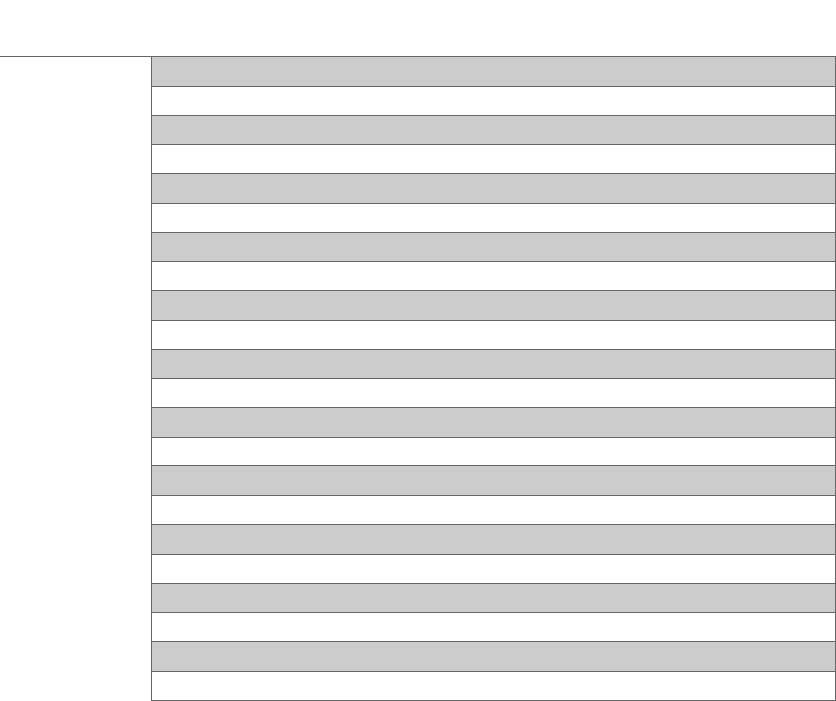
Figure 11: Derived hull lines plan.
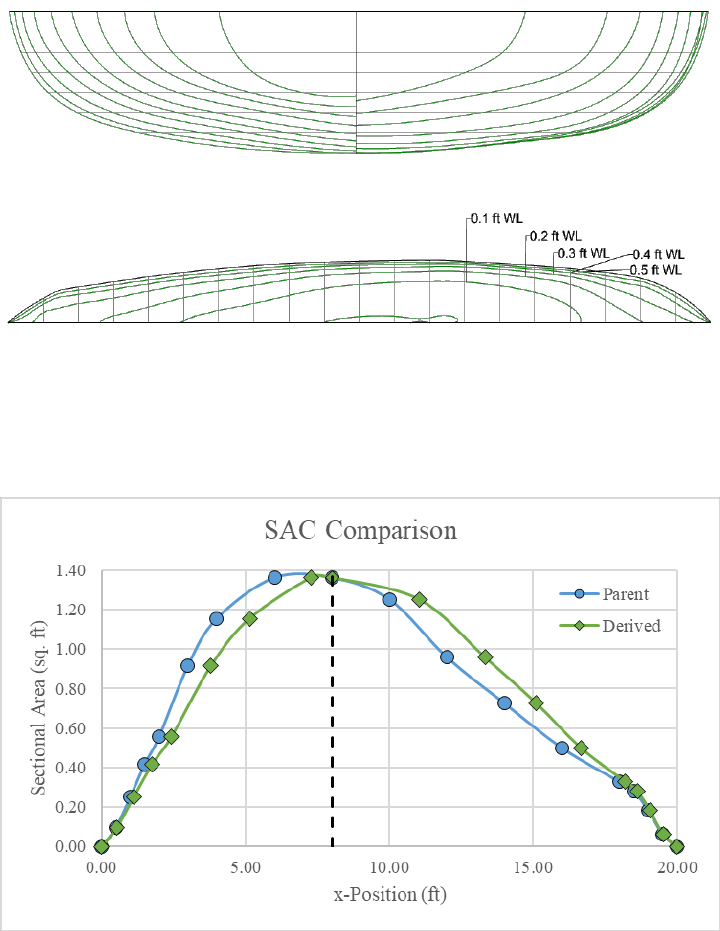
Figure 12: Comparison of parent and derived hull sectional area curves.

30
Placing the sectional area curve of the derived hull over top the parent hull, the effect of the
Lackenby shift becomes visible. Since the midship, forward extent of the parallel midbody, and
aft extent of the parallel midbody all lie on the 8ft station, a parallel midship cannot be added as
there is only one station that would have to move to two locations. This could be fixed by updating
the variable definitions in the code, but currently, adding a parallel midship to a vessel that does
not originally have one is impossible. Importantly, the Lackenby shift has been executed as
described. The forebody areas have increased and aftbody areas decreased according to the
specified forward shift of the LCB. While it is hard to analyze visually whether the overall volume
has increased, thus far nothing appears amiss with the data.
Figure 13: Comparison of parent and derived hull body plans.

31
By overlapping the body plans of the parent and derived hulls we can analyze the changes
present in the derived hull form. The top part of Figure 13 shows stations 0-10 for the parent hull
(blue) and the derived hull (green) and the bottom part shows stations 11-20. The changes in
volume observed in the sectional area curve are reflected in the body plan. For every station aside
from midship, forward perpendicular, and aft perpendicular, the cross-sections of the derived hull
stations are larger for the forebody and smaller for the aftbody compared to the parent hull.
Comparing the variables calculated for the Lackenby shift of the parent hull with the values
of the derived hull can also offer valuable insight.
Table 6: Comparison of half-body variables.
Variable
Units
Parent Hull
Derived Hull
Forebody Variables
iparallel
-
8
8
L
ft
12.00
12.00
CP
-
0.5454
0.6053
xLCB
ft
4.1586
4.2825
k
ft
5.0860
5.1647
R
ft
5.7766
5.8213
theta
rad.
-0.1258
-0.1296
Aftbody Variables
iparallel
-
8
8
L
ft
8.00
8.00
CP
-
0.6914
0.6186
xLCB
ft
2.9631
2.8314
k
ft
3.5062
3.3953
R
ft
3.9037
3.8128
theta
rad.
0.1906
0.1789
Other Variables
AM
ft
2
1.3614
1.3614
V
ft
3
16.4395
16.6248
CP
-
0.6038
0.6106
xLCB
ft
0.8966
1.3998
32
First thing of note is that the sign of every value matches expectations, particularly the entrance
angle of the forebody is negative and the run angle of the aftbody is positive. This matches the
orientation of the vessel in Rhino (and the stations defined in the CSV file) with the aft
perpendicular laying on the origin and the vessel pointing forward into the positive x-axis. Next,
iparallel for each half-body of the parent and derived hull is equal and constant. This is
expected as the sample vessel has no parallel midship, so the index marking the extent of the
parallel midship for all half-bodies will be equal to the index of the midship station. The half-
bodies of both the parent and derived hulls are equal and add up to the LPP, which is accurate as
no changes were made to add a parallel midbody. The midship area, AM, also remains identical
between both vessels, which matches theory as midship is one of the stations unaffected by the
Lackenby shift. Additionally, the data confirms the execution accuracy of the Lackenby shift
observed visually prior. The prismatic coefficient and LCB of the forebody increased and,
conversely, the same variables decreased in the aftbody. Furthermore, the overall LCB, volume,
and prismatic coefficient of the vessel increased according to the input values.
However, despite the simplification that set the parent and derived half-body slopes equal,
the calculated slope has changed slightly for both half-bodies. This is due to the method used to
calculate the slopes. The extent of the slope was defined and calculated using the two consecutive
points at the vessel extremities; however, when the station locations are shifted, the x-values used
when calculating the slope of the curve are now different.
33
6. Conclusions
In conclusion, this project successfully demonstrated the feasibility of automating a
Lackenby shift with McNaull’s expansion using Rhino’s scripting tools. Given the limitations of
the testing vessel, the auxiliary scripts and the user interface worked as expected and the main
script easily allows a user to create a model of a derived hull form in Rhino with minimal
interaction. The current version of this code is restricted in its practical applications; however,
there is ample room for improvement and expansion.
The script currently requires a CSV file input and can only perform a shift on a symmetrical
hull form free of appendages. In order to further improve the ease-of-use of this script,
offsetimport.py needs to be generalized to allow for point cloud or station imports from Rhino,
General Hydrostatics (GHS), or other formats. This would encourage engineers to use the program
as they could more easily modify a working hull model for use with the script. The cubicmatrix.py
auxiliary script should be further developed to allow the bow and stern angles of the derived hull
to be defined or calculated separate from the parent hull.
Additionally, appendage compatibility could be added to broaden the applicability of the
script. For example, a Lackenby shift of a bulbous bow could be applied fairly easily. Everything
forward of the forward perpendicular (FP) could be considered part of the bulbous bow, the cross-
sectional area of the hull at the FP would be the cross section of the bulb, and the FP itself would
be the “midship” of the bulb. If overall size changes were desired, the bulb could be stretched
horizontally or vertically by modifying the station spacing or design draft defined by the user. The
user could specify these modification ratios along with the bulb length and centroid of the parent
hull. With this information, a Lackenby shift of a bulbous bow could be performed.
34
However, before considering additional features and capabilities, the current iteration of
the code should be tested with simple hull form containing a parallel midship to prove that the
Lackenby shift is being executed properly. To achieve this, definitions used to calculate the data
of the derived hull form should be modified to properly execute a Lackenby shift regardless if the
vessel has or is modifying a pre-existing parallel midship. With the above modifications and
expansions, the script has potential to become a very comprehensive modeling tool. In concert
with other Rhino tools such as Orca and Grasshopper, this script could even be used for rapid
preliminary hull design testing. A number of potential hull models could be developed from a
single parent hull and optimized for resistance and propulsion or a number of other design
objectives.
35
References
Akima, Hiroshi. "A New Method of Interpolation and Smooth Curve Fitting Based on Local
Procedures." Journal of the ACM (1970): 589-602. Electronic Document.
Birk, Lothar. "A Comprehensive and Practical Guide to the Hess and Smith Constant Source and
Dipole Panel." Ship Technology Research (2021): 50-62. Document.
Bole, Marcus. Parametric Generation of Yacht Hulls. Final Year Project. Glasgow: University of
Strathclyde, 1997. Electronic Document.
Harries, Stephan. Parametric Design and Hydrodynamic Optimization of Ship Hull Forms. PhD
Thesis. Berlin: Technische Universität Berlin, 1998. Electronic Document.
Lackenby, H. "On the Systematic Geometrical Variation of Ship Forms." Trans. INA (1950): 289-
316. Electronic Document.
McNaull, Robert. "Generating New Ship Lines from a Parent Hull Using Section Area Curve
Variation." REAPS Technical Symposium. Philadelphia: U.S. Department of the Navy,
1980. 337-369. Document.
Meier, Mark. "Meier_UI_Utility.py." Easily Create Graphical User Interfaces in Rhino Python. 3
December 2012. http://mkmra2.blogspot.com/2012/12/creating-graphical-user-interfaces-
with.html?q=UI.
Taylor, D. W. The Speed and Power of Ships: A Manual of Marine Propulsion. Washington, D.C.:
Press of Ransdell, Inc., 1933.
36
Appendix A
Details:
This report, intended for readers more familiar with programming, details how the auxiliary scripts
and user interface were developed and structured.
Filename:
NAME 6093 Report - Details on the Auxiliary Scripts and User Interface.pdf
37
Appendix B
Details:
Comma-separated values (CSV) file containing offsets for four geometric ship-like sections used
within the auxiliary file secarea.py to test the functions of offsetimport.py, secarea.py, and
akimaint.py.
Filename:
offsets_areatest.csv
38
Appendix C
Details:
Rhinoscript file that uses the auxiliary files to complete the Lackenby shift of the underwater body
of a hull using station offsets provided in CSV file format. The file is executed within Rhino’s
script editing window.
Filename:
main.py
39
Appendix D
Details:
CSV file containing offset values for a generic kayak, used to demonstrate the functionality of
main.py. The offsets are defined with stations, half-breadths, and elevation values with the forward
perpendicular (station 0) at the origin. Half-breadth values are defined as a fraction of the
maximum half-breadth and elevation values are defined as a fraction of the design waterline.
Filename:
offsets_kayak.csv
40
Appendix E
Details:
Text file containing the program description, conditions, instructions usage guide, and credits for
main.py and all accompanying auxiliary files.
Filename:
readme.txt
41
Appendix F
Details:
Python script written by Dr. Lothar Birk, University of New Orleans. Defines a function that takes
a series of coordinate points split into two arrays and performs Akima interpolation on them. Also
contains a test portion that demonstrates the functionality of the script.
Filename:
akimaint.py
42
Appendix G
Details:
Python script that defines the cubic matrix used for McNaull’s expansion of the Lackenby method.
Filename:
cubicmatrix.py
43
Appendix H
Details:
Python script written by Dr. Lothar Birk, University of New Orleans. Defines a function containing
a simple Gaussian elimination algorithm. Also contains a small test script used to demonstrate
usage of the function.
Filename:
gauss.py
44
Appendix I
Details:
Python script written by Dr. Lothar Birk, University of New Orleans. Defines a function to import
station data from a CSV file and convert the data into coordinate points separated by station into a
series of arrays.
Filename:
offsetimport.py
45
Appendix J
Details:
Python script containing functions for calculating sectional area, area moments, second order
moment of volume, and third order moment of volume. Also contains section used to test the
functionality of akimaint.py, offsetimport.py, and the functions defined within secarea.py.
Filename:
secarea.py
46
Appendix K
Details:
Contains the station offsets, SAC, and Lackenby shift data for the sample parent hull used
introduced in Section 4.
Filename:
LackenbyShift_ParentHull.dat
47
Appendix L
Details:
Contains the station offsets, SAC, and Lackenby shift data for the derived hull form discussed in
Section 5, found from the sample vessel introduced in Section 4.
Filename:
LackenbyShift_DerivedHull.dat
48
Vita
The author was born in Seattle, Washington. She obtained her Bachelor’s degree in naval
architecture and marine engineering from the University of New Orleans in 2021. She continued
to pursue a Master’s degree in naval architecture and marine engineering from the University of
New Orleans, working with Dr. Lothar Birk on the automation of hull design using programming.
