
1
Introduction
BARS relies heavily on interoperability with Microsoft Excel to provide users with an alternative
view of data and an alternative form of data entry. Users can export different grids within each of
the BARS tabs to Excel and can use those exports to do massive data entry for eventual
upload/import. Pivot tables bring the capabilities of Excel and BARS a step further, allowing users
to dig deeper into what information is being provided by BARS to make better decisions in
adjustments.
This training is not meant to cover all aspe
cts of using Microsoft Excel or pivot tables, but will
provide new users with several basic key instructions and features to get started. This training will
work through an instructional scenario using the BARS system.
Step 1:
Log into BARS Production
Step 2:
From the BARS Homepage/Worktray, hover over Operating Budget at the top of the page and
select Adjustments > Agency / OBA Adjustments.
Step 3:
Complete Overview Tab with all of the required information.
Once the Overview Tab i
s complete, move to the Expenditures Tab.

2
Step 4:
In the Expenditures Tab—
Confirm the information brought over from the Overview Tab is correct in the top section, and
select the magnifying glass next to the Expenditure Sub-Program Filter to bring up a window to
select a specific unit, program, or subprogram of the selected agency.
Click on that program or subprogram to highlight that portion of the budget. Once you have
highlighted all of the desired units, programs, and subprograms, select Accept Selection to ready
those sections of the budget to be loaded.
To then load the Expenditure Financials grid below, click Load Sub-Program Expenditures.

3
Step 5:
Once the Expenditure Financials grid has been populated, scroll down to view the grid.
As shown below, the Expenditure grid has been populated with the data that is already in BARS
through uploads and prior year adjustments. As mentioned in the “Creating an Adjustment” guide,
adjustments may be made in the system in the “FY 20XX Adjustment” column or the “Export” and
“Import” functions.
Scroll to the bottom left of the grid and select the Export button.
This will bring up a separate window that that saves the document (depending on the user’s
download settings) and requires the user to open the file.
Open that file.
Step 6:
In the Excel Spreadsheet—
Confirm that the information exported by the system is the data for the selected agency, unit,
program, and subprograms as selected in Step #4. If the warning message appears, the user must
click Enable Editing before proceeding with the instructions below.

4
Step 7:
Once the spreadsheet is unlocked for editing, begin by using the “Filter” tool to create a column-
by-column filter of the information out of BARS.
1. Highlight all of Row 1 of the spreadsheet.
2. Find the “Sort & Filter” tool at the top-right of the Home tab in Excel.
3. Select “Filter”
This will insert a filter for each column of the current spreadsheet, with the filter running off of
Row 1 of each column. After clicking the downward arrow in the “Object” column, a list of

5
checkboxes of the column’s text contents will pop up. This list of checkboxes can be used to
include or hide lines with these categories in the spreadsheet.
Filter the spreadsheet to display only Object 09 and 10.
Users can use this tool to look specifically at individual programs, a list of subprograms, single
objects, or even filter out all lines that are “$0” in in a given fiscal year.
Note: Users may also sort data using this feature.
Step 7:
Now that the spreadsheet has been filtered for Object 09 and 10, use the “Freeze Pane” tool in
Excel to freeze chart of accounts data to the left of the spreadsheet.
1. Highlight all of the columns that contain data and double-click on the margins between the
columns (where it says “A, B, C…”). This will change the width of the columns such that no
headers or data is hidden. By clicking in the margins of the columns, individual column
widths may also be narrowed or expanded.

6
2. Click into the first cell that does not need to be frozen. For this exercise, it would be cell
H2. Find the “View” tab, select “Freeze Panes” to open the drop-down menu, and click
Freeze Panes. All columns from H and rightward will scroll with the rest of the page.
Step 8:
Once the panes have been frozen, scroll to the right to the “FY 20XX Current” column (Column N
in the example).
This column contains the current dollars in the system tied to each of those line items. Without
action in the “FY 20XX Adjustment” (Column O in the image) in the form of added (positive) or
subtracted (negative) dollars, nothing will be changed by the adjustment. Individual dollar
amounts can be entered into this column to add or subtract to the existing values.
For more advanced tools for Excel, Step #9 shows the use of formulas to augment existing budget
data.
Step 9:
With Objects 09 and 10 selected, go to the “FY 20XX Adjustment” column and click into the very
top empty cell. As a tool, Microsoft Excel can grab data from one cell and manipulate it in another
cell, called a “formula.” This walkthrough will create two sample formulas.
Placeholder for Inflation
1. Click into that top-most empty cell in the “FY 20XX Adjustment” column in Column O. For
the example above, that is cell O41.

7
2. Type directly into the cell “=” and the directly adjacent cell in the “FY 20XX Current”
column in Column N.
3. Once the cell has been selected, use the keyboard to type in the following formula “
*.03”. For the above example, that would be “=N41*.03”.
4. Press enter.
5. Click and hold the small green square in the bottom right corner of the frame surrounding
the newly formulated value, and double-click or drag that icon all the way down to the
end of the line item data shown. This will take the formula created in the original cell
(O41 as shown above) and translate it to the remaining line items. This action allows
formulas to be calculated across multiple lines, as might make sense when accounting for
inflation in the FY 2021 agency budget request.

8
6. Clean up decimals so that only whole numbers remain. This can be done by overwriting the
formula in the cell with the new number or going a step further and adding a rounding
formula into the equation, and then dragging that formula down again.
- Or -
7. Confirm that the information makes sense for the agency request.
Intra-agency Target
1. If a given unit or program is provided with a target by a central budget office within an
agency, Excel can be used to evenly or proportionally disperse specific amounts among
existing line items. Begin by entering the amount to be dispersed at the bottom of the row
of line items in the “FY 20XX Adjustment” column (Column O).

9
2. Next, sum the shown rows in the “FY 20XX Current” column at the bottom of the row of
line items (Column N). This may be performed through the “=SUM” formula in Excel, shown
below.
3. To disperse the provided target ($10,000), in the “FY 20XX Adjustment” column multiply
that target by the proportion of the line item to the sum. Begin by selecting the top-most
line item. You may also add in the rounding formula to shortcut any rounding issues.
4. Once this formula has been calculated for the top-most cell, repeat this formula for each
of the cells below holding the “total value” cells constant. This can be achieved by adding
a “$” in front of the row number for the formula in the top-most cell, and copying and

10
pasting the formula to each of the cells below. Again, this action allows formulas to be
calculated across multiple lines, as it might make sense when accounting for an intra-
agency target in your agency’s budget request.
5. Confirm that the data produced by the formula makes sense, and then copy and paste the
“FY 20XX Adjustment” column data “as value” back into its location.
6. Delete the row with the “total value” cells (row 59 as shown above). Deleting these
rows/cells should not affect the newly-created adjustment line-item detail created by the
formula if the “copy and paste” action above was performed properly.
Note: Detail may be added into the empty section of the workbook, but may create extraneous
detail in the import if not deleted. Tidying up the workbook prior to upload will reduce the
chance of data issues with the import.
Step 10:
Once the adjustment values have been included in the “FY 20XX Adjustment” column and all
extraneous data has been removed, the worksheet is ready for upload as an import file. However,
Excel can also be used as a tool for advanced analysis for the budget and its complex data. By
creating “Pivot Tables” the user can easily organize and analyze the data of their budget. This can
be used to great effect to inform a single adjustment.
11
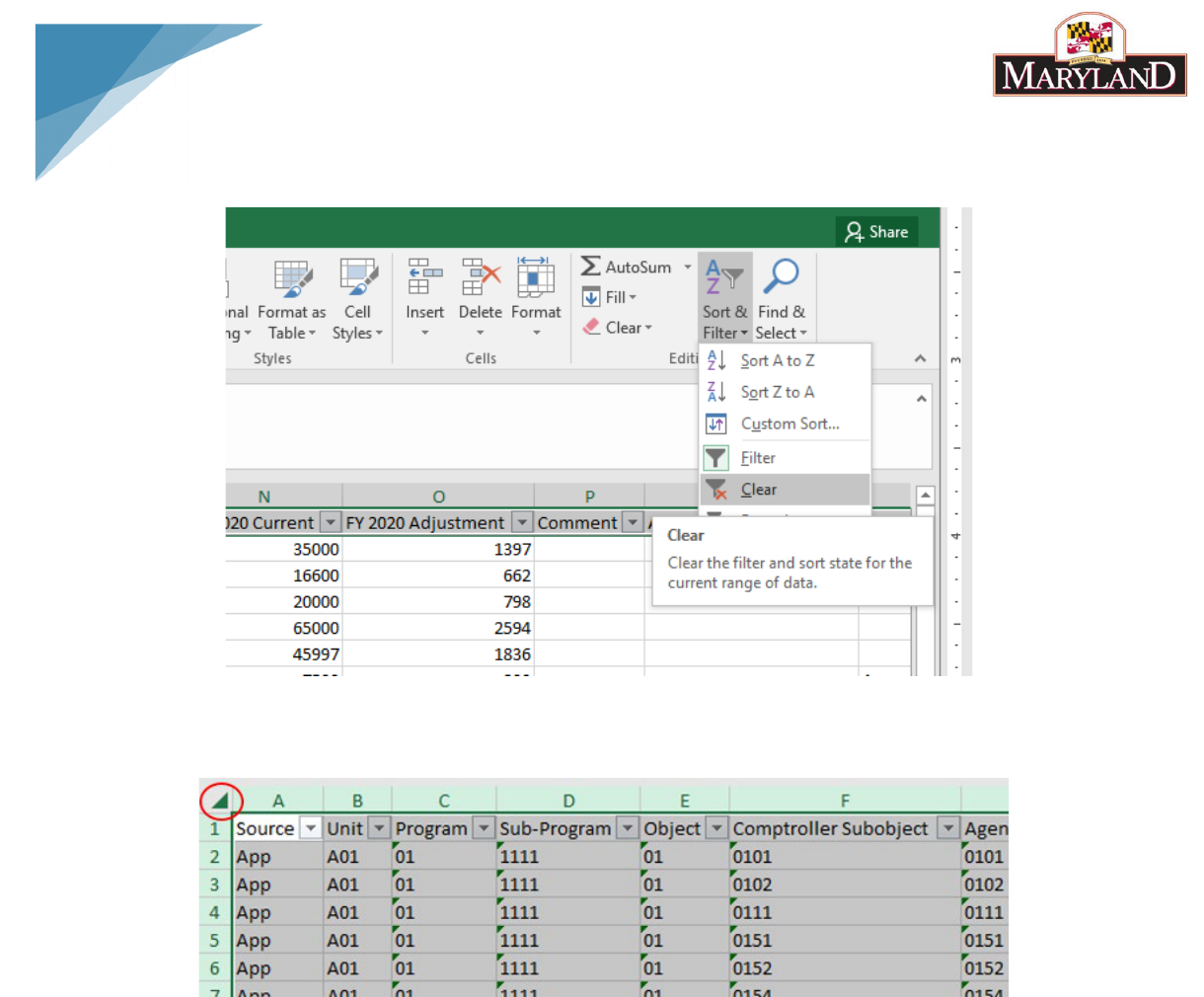
Clear the filter of the grid by highlighting the top row of the worksheet and using the “Clear”
function. This can be found in the “Home” tab under the same “Sort & Filter” tool.
Click on the “arrow” icon at the top left of the worksheet grid. This arrow allows the user to
“Select All” data currently within the grid.
Once all of the data has been selected, go to the “Insert” tab at the top of the Excel page and
click into the “PivotTable” tool.

12
If you have successfully used the “Select All” function, clicking this “PivotTable” button will bring
up a dialogue box with the data pre-selected in the “Select a table or range” field. Click “OK.”
This will create a separate worksheet in the Excel workbook with the beginning framework of a
Pivot Table in a new worksheet named “Sheet1.”

13
Step 11:
In “Sheet1,” find the following window embedded in the grid, marked “A” above.
This space represents the “canvas” for the beginning of the Pivot Table. Begin by adding pieces of
the dataset from section “B” (by either dragging them into one of the four layout boxes or clicking
on the checkbox and adjusting from there) marked above. Pivot tables allow users to create
customizable spreadsheets that incorporate data from the original worksheet as shown in the
example below:

14
Section B is broken up into five main parts:
Fields: Each of these “fields” represents a column header from the source spreadsheet. In the
above example, each of the fields are the direct column headers found in the Expenditures grid in
BARS and represent a mocked-up line item adjustment summary.
Filters: Fields dragged into this box create an overarching filter that allows data to be pre-
selected and adjusted based on the needs of the user. Multiple fields can be added into this piece
the layout, such as “Object” as shown in the above example which has been filtered to only show
Objects 09 and 10.
Rows: Fields dragged into this box divide up the displayed data as independent factors in the
reporting. The fields in the “Rows” layout box represent the data inputs which ultimately produce
the data outputs in the “Values” layout box. As shown in the example above, “Unit,” “Program,”

15
“Sub-Program,” and “Comptroller Subobject” have been selected to display the familiar line item
detail structure found in the original worksheet as well as the Expenditures tab in BARS.
Values: Fields dragged into this box represent filters on the dependent factors in the reporting.
The Fields in the “Values” layout box represent these data outputs based on the layout created in
the “Rows” layout box. As shown above, a three-year summary of the data has been selected in
order to display the baseline for the data as it exists in BARS, as well as the “FY 2020 Adjustment”
column, which provides a clear summary of all line item adjustments from the source worksheet.
Columns: Fields dragged into this box divide up the displayed data based on type, such as
“Dollars” or Adjustment “Stage” or “Status” in the case of certain data pulled from BARS. Based
on certain detail dragged into the “Values” layout box, this box will automatically populate with
the column type most appropriate for that selection. In the example above, it has automatically
populated to show the sum values of the filtered data.
Step 12:
By simply dragging the above sections into the displayed layout boxes, the overarching design of
the pivot table may still leave clarity to be desired. Replicating the above layout boxes results in
the following design:

16
By using “Design” elements and adjusting “Value Field Settings” users can create a more familiar
format in their pivot tables.
Begin by selecting the “Design” tab at the top of the Excel screen under “PivotTable Tools” and
select “Show in Tabular Form” and “Repeat All Item Labels” under the Report Layout drop down
menu. This will design the layout of the data such that data is repeated for each line and each
“Row Label” receives its own discrete column.
Then, under the Subtotals drop down menu select “Do Not Show Subtotals” to eliminate individual
subtotals running off of each chart of accounts selection in the “Rows” layout box.

17
By using these two quick design changes, users can transform the data to read in a line-item
fashion.
Step 13:
Once the design elements have been adjusted, right-click into the column titled “Count of FY
2020 Adjustment” and select “Value Field Settings…”
This will bring up a window that allows the individual column to be adjusted to the preferences of
the user. Columns can be renamed and fields can be summarized differently. Rename the column
to “2020 Adjustments” and select “Sum” under the “Summarize value field by” window and press
OK.
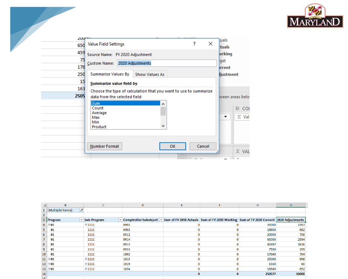
18
By making this change to the value field, the data in the “2020 Adjustments” column will now
report data the same way as the individual fiscal year columns, as a “Sum.”
The finished product should ultimately look like the following:
