
Agilent Technologies
Aria Real-Time PCR
Software
User Manual
Revision J1, September 2023
AriaMx: For Research Use Only. Not for use in
diagnostic procedures.
AriaDx: For In Vitro Diagnostic Use
Always make sure you are using the most recent version of the Aria software. Check the
Aria software download website at www.agilent.com/en/ariamx-software-download.
Agilent Aria Real-Time PCR Program 2
1 Getting Started with the Aria Software 14
The Aria software 15
Getting Started with the Aria Software 16
Introduction to the Aria software 16
Overview of the user interface 18
Home screen 18
Menu toolbar 18
Tabs 18
Left and right panels 18
Home/Notifications/Help icons 19
Getting Started screen 19
Experiment Notes / Project Notes 19
Help access for the Aria software 20
Help system 20
Sample experiments 21
2 Specifying Hardware and Software Settings 22
Update instrument optics 23
Change the default crosstalk correction settings 25
Set software preferences 28
Set default file name configuration 28
Create and apply analysis templates 29
3 Performing Hardware and Software Tests and HRM Calibrations 32
Run an instrument qualification test 33
Run the test 33
About the Qualification Test graphical data 34
Perform an Installation Qualification test 36
Run an HRM calibration plate (HCP) 38
Prepare the plate 38
3 Agilent Aria Real-Time PCR Program
Run an HCP 39
If the HCP fails 40
4 Creating/Opening an Experiment 42
Overview of the Getting Started screen 43
Tools available on the Getting Started screen 44
About the Aria file types 45
Quick Start Protocol 46
How to create, set up, run, analyze, and generate reports for an experiment 46
Create a new experiment 49
Create an experiment based on experiment type 49
Create an experiment from a template 50
Create an experiment from a LIMS data file 51
Open an existing experiment 53
Save a copy of an existing experiment 54
Create a template from an existing experiment 55
Convert an experiment to a new experiment type 56
5 Selecting an Experiment Type 58
Overview of Experiment Types 59
Quantitative PCR 59
Comparative Quantitation 59
Allele Discrimination - Fluorescence Probes 60
Allele Discrimination - DNA Binding Dye with High-Resolution Melt 60
User Defined 60
The Quantitative PCR Experiment Type 61
Multiplexing quantitative PCR experiments 61
Well types for Quantitative PCR experiments 62
The Comparative Quantitation Experiment Type 63
Normalizing chance variations in target levels 63
Agilent Aria Real-Time PCR Program 4
Determining amplification efficiencies for the targets of interest and normalizer targets 64
Including biological replicates in comparative quantitation 65
Well types for Comparative Quantitation experiments 66
The Allele Discrimination - DNA Binding Dye Experiment Type 67
About HRM calibration plates 67
Well types for Allele Discrimination - DNA Binding Dye experiments 68
The Allele Discrimination - Fluorescence Probe Experiment Type 69
Well types for Allele Discrimination - Fluorescence Probe experiments 70
The User Defined Experiment Type 71
6 Setting Up the Plate 72
Overview of the Plate Setup screen 73
The plate map 74
Well type 74
Well name / Sample name 74
Target information 75
Replicate number 75
Reference dye 75
The Properties panel 76
Additional tools for setting up a plate 76
Import a plate setup 78
Select and view wells in the plate map 79
Select wells in the plate map 79
Unselect wells in the plate map 80
View details of a well or wells 80
Export the plate map image 85
Assign plate properties for a Quantitative PCR DNA Binding Dye experiment 86
Assign well types 86
Assign well names 86
Assign dyes/targets 88
Select a reference dye 89
5 Agilent Aria Real-Time PCR Program
Assign replicates 90
Assign quantities to Standard wells 92
Assign plate properties for a Quantitative PCR Fluorescence Probe experiment 94
Assign well types 94
Assign well names 94
Assign dyes/targets 96
Select a reference dye 97
Assign replicates 98
Assign quantities to Standard wells 100
Assign plate properties for a Comparative Quantitation experiment 102
Assign well types 102
Assign well names 103
Assign sample names and biological replicates 104
Assign dyes/targets 107
Select a reference dye 108
Designate the normalizer 108
Assign replicates 109
Assign quantities to Standard wells 111
Assign plate properties for an Allele Discrimination DNA Binding Dye experiment 113
Assign well types 113
Assign well names 113
Assign sample names 115
Assign dyes/targets 117
Select a reference dye 118
Assign replicates 119
Assign plate properties for an Allele Discrimination Fluorescence Probe experiment 122
Assign well types 122
Assign well names 122
Assign sample names 124
Assign dyes/targets 126
Select a reference dye 127
Assign Alleles 128
Agilent Aria Real-Time PCR Program 6
Assign replicates 128
Assign plate properties for a User Defined experiment 131
Assign well types 131
Assign well names 131
Assign sample names and biological replicates 133
Assign dyes/targets 135
Select a reference dye 137
Designate the normalizer 137
Assign Alleles 138
Assign replicates 138
Assign quantities to Standard wells 141
7 Setting Up the Thermal Profile 142
Set up the thermal profile 143
Elements of a Thermal Profile 144
Import a thermal profile 146
Edit the thermal profile 147
Export the thermal profile image 159
8 Running and Monitoring Experiments 160
Overview of the Instrument Explorer dialog box 161
Add instruments to your network 162
Add a new instrument based on its IP address 162
Add a new instrument based on its port number 163
View information about an instrument 163
Start, stop, or pause a run 165
Start a run 165
Cancel a run 166
Pause a run 167
Monitor a run 168
Connect to the running instrument 168
7 Agilent Aria Real-Time PCR Program
Monitor a run by viewing its progress through the thermal profile 169
Monitor a run by viewing the raw data plots 169
Change the display options for the raw data plots 170
Stop monitoring a run 172
Retrieve run data from the instrument 173
Retrieve data through the network 173
Retrieve data using a USB drive 174
Export instrument data to a CSV file 175
Export instrument data by column 175
Export instrument data by target 175
Export instrument data by wells 175
9 Setting Analysis Criteria 176
Overview of the Analysis Criteria screen 177
Toggle display of plate map wells 178
Select the wells and well types to include in analysis 179
Select wells for analysis using the plate map 179
Select wells for analysis based on well type 179
Select the targets to include in analysis 180
Select which data collection points to analyze 181
Choose a treatment for replicate wells 182
Assign an HRM calibration plate 183
Assign an HCP for new experiments 183
Assign an HCP using the HCP icon 184
10 Viewing Graphical Displays of the Results 186
Overview of the Graphical Displays screen 187
Graphs 187
Result table 188
Display options 188
Agilent Aria Real-Time PCR Program 8
Zooming 190
Configure and apply analysis templates 192
Configure an analysis template in the Analysis Term Settings dialog box 193
View the Amplification Plots 197
View data for a single data point 197
Select a fluorescence data type 198
Specify the use of smoothing 198
Adjust the graph properties 199
Adjust the baseline correction settings 199
Adjust the crosstalk correction settings 201
Select the scale (linear or log) of the Y-axis 206
Manually adjust threshold fluorescence values 207
Adjust threshold fluorescence values by altering the algorithm settings 209
Lock or unlock the threshold fluorescence values 210
View the Melt Curve - Raw/Derivative Curve 212
About raw/derivative curves 212
View data for a single data point 213
Select a fluorescence data type 213
Adjust the graph properties 214
Specify the use of smoothing 214
Normalize the fluorescence values 214
Adjust the range of the X-axis 215
Adjust product melting temperature settings 216
View the Melt Curve - Difference Plots 218
About difference plots 218
Select a fluorescence data type 220
Assign the control target 220
View data for a single data point 221
Manually assign Unknowns to a genotype call 221
Adjust the graph properties 224
View the Standard Curve 225
9 Agilent Aria Real-Time PCR Program
View data for a single data point 225
Select a fluorescence data type 226
View the R-squared values, slopes, and amplification efficiencies 227
Adjust the graph properties 228
Manually adjust threshold fluorescence values 228
Display and adjust confidence intervals 229
View the Relative Quantity 230
About relative quantities 230
Select a fluorescence data type 231
Set the Y-axis scale for the Relative Quantity chart 231
Add error bars to the Relative Quantity chart 232
Adjust the graph properties 232
Select the algorithm method 232
Enter the amplification efficiencies for the targets 233
View the Allele Determination graph 235
View data for a single data point 235
Select data type and fluorescence type to display 236
Display genotype groups on the graph 237
Adjust the graph properties 238
Adjust the last cycle 238
Rename the genotype groups 239
Customize graph properties 240
Customize graph properties using the short-cut menu 240
Customize graph properties using the Graph Properties dialog box 243
11 Generating Reports and Exporting Results 252
Generate report of results 253
View a preview of the report 253
Select report type 253
Generate the report 253
Configure the report 254
Create or edit report configuration definitions 257
Agilent Aria Real-Time PCR Program 10
Export data/results to an Excel, text, LIMS data, or RDML file 260
Configure the file and export data 260
Load a saved data export definition 264
Create or edit data export definitions 265
12 Creating and Setting Up an MEA Project 268
Quick Start Protocol 269
How to create, set up, analyze, and generate reports for a multiple experiment analysis
project 269
Overview of multiple experiment analysis 270
Applications 270
Restrictions 271
Guidelines for Comparing Cq Values Across Experiments 272
Reducing plate-to-plate variability 272
Selecting a method for setting threshold fluorescence levels 273
Create an MEA project 275
Open an existing MEA project 276
Select experiments for a project 277
Add or remove experiments from the project 277
Include or exclude experiments in the project analysis 278
Edit the plate setup of experiments in a project 279
Select an experiment to edit 279
Differentiate between targets across experiments 279
Edit plate properties 280
View the thermal profiles of experiments in a project 281
13 Analyzing Multiple Experiment Analysis Project Results 282
Set analysis criteria for a project 283
Toggle display between one experiment and all experiments 283
Select the wells and well types to include in analysis 283
Select the targets to include in analysis 284
11 Agilent Aria Real-Time PCR Program
Select which data collection points to analyze 284
Choose a treatment for replicate wells 285
Overview of the Graphical Displays screen for a project 286
Graphs 286
Result table 287
Display options 287
Zooming 289
Compare amplification plots in a project 291
Compare amplification plots by experiment 291
Compare amplification plots by target 291
Consolidate the amplification plots 292
Compare raw or derivative melt curves in a project 293
Compare raw or derivative melt curves by experiment 293
Compare raw or derivative melt curves by target 294
Consolidate the raw or derivative melt curves 294
Compare standard curves in a project 295
Compare standard curves by experiment 295
Compare standard curves by target 296
Consolidate the standard curves 296
Compare Relative Quantity charts in a project 297
Compare relative quantities by experiment 297
Compare relative quantities by target 298
Consolidate the relative quantities 298
Compare Allele Determination graphs in a project 299
14 Generating Multiple Experiment Analysis Reports and Exporting Results 300
Generate report of MEA project results 301
View a preview of the report 301
Select report type 301
Generate the report 301
Configure the report 302
Agilent Aria Real-Time PCR Program 12
Create or edit report configuration definitions 305
Export MEA data/results to an Excel, text, or LIMS data file 308
Configure the file and export data 308
Load a saved data export definition 311
Create or edit data export definitions 312
15 “How-To” Examples for Multiple Experiment Analysis Projects 314
Example 1 315
How to find the initial template quantity of a target in an unknown sample using a standard curve
from a separate experiment 315
Example 2 317
How to normalize target quantities in Unknown and Calibrator wells using a normalizer target from a
separate experiment 317
16 Help for the Aria ET (Electronic Tracking) Software 320
Overview of the Aria ET software 321
Open an experiment in the Aria ET software 323
Open an experiment 323
Import and export experiments in the Aria ET software 326
Import experiments into the database 326
Export experiments from the database 326
Lock or log out of the Aria ET software 328
Lock the program 328
Log out of the program 328
Change your password in the Aria ET software 330
Create a multiple experiment analysis project in the Aria ET software 331
Manage users in the Aria ET software 332
Set account properties for all users 332
Manage user accounts 335
Archive and restore experiments in the Aria ET software 339
13 Agilent Aria Real-Time PCR Program
Archive experiments 339
Restore experiments 341
View audit trails and system logs in the Aria ET software 343
View the audit trail logs 343
View the system logs 346
Add and remove databases in the Aria ET software 348
Add an Aria ET database 349
Remove an Aria ET database 350
View transaction logs in the Aria ET software 352
View transaction logs for primary database 352
View transaction logs for an archive database 353
17 Reference Help and Troubleshooting & Support 354
QPCR Glossary 355
Experiment Type and QPCR Detection Chemistry Terms 355
Well-Types 357
Analysis Terms 358
LIMS File Format for Aria Software 361
Plate Setup 361
Experiment Setup 363
Thermal Profile 363
Default Optical Module 364
Threshold Fluorescence 364
Trademarks 366
Troubleshooting and Support 367
Troubleshooting Guide 367
Contact Agilent Technical Support 370

Agilent Technologies
1
Getting Started with the Aria Software
The Aria software 15
Getting Started with the Aria Software 16
Introduction to the Aria software 16
Overview of the user interface 18
Home screen 18
Menu toolbar 18
Tabs 18
Left and right panels 18
Home/Notifications/Help icons 19
Getting Started screen 19
Experiment Notes / Project Notes 19
Help access for the Aria software 20
Help system 20
Sample experiments 21
1 Getting Started with the Aria Software
The Aria software
15 Agilent Aria Real-Time PCR Program
The Aria software
The Aria software features a variety of experiment type options with
customized plate and thermal profile setup, and experiment analysis
screens that streamline the process of collecting and analyzing data for
specific applications. The software capabilities allow you to:
• Quickly set up an experiment using a template or the Import Plate
Setup function
• View raw fluorescence data without mathematical correction or
calibration factors
• Quantitate the initial template quantity of a DNA target based on a
standard curve
• Generate and display normalized relative quantity values on a log(2)
fold change chart to assess the effects of an experimental treatment on
gene expression levels
• Export any data set directly to Microsoft Excel or to a text file
• View and analyze the data from several experiments together in a single
project using the multiple experiment analysis functions
• Use high resolution melt analysis for SNP genotyping in an Allele
Discrimination experiment

Getting Started with the Aria Software 1
Getting Started with the Aria Software
Agilent Aria Real-Time PCR Program 16
Getting Started with the Aria Software
Introduction to the Aria software
The software's Home screen provides an introduction to the program and
a list of program features.
To open the Home screen: Click the Home icon near the upper right
corner of the program window.
NOTE
NOTE
If you want the program to open to the Home screen, mark the check box near the
bottom of the screen labeled Show Home on StartUp.

1 Getting Started with the Aria Software
Getting Started with the Aria Software
17 Agilent Aria Real-Time PCR Program
Introduction
To view the Introduction, click Introduction (near the top right corner of
the Home screen). The text on this screen provides an overview of the
AriaMx/AriaDx Real- Time PCR System.
Features
To view the Features, click Features (near the top right corner of the
Home screen). The text on this screen lists the features of the Aria
software.
Minimum PC requirements
Table 1 lists the minimum PC requirements needed to run the Aria
software.
* Installers for Microsoft .NET Framework 4.0 and Microsoft SQL Server 2019 are provided
on the Aria Software Download page of the Agilent website. If you do not have the needed
Microsoft Visual C++ 2010 components, then the Aria installer will automatically install
them to your PC when you initiate installation of the Aria software.
Table 1 Minimum requirements for running the Aria software
Operating system Windows 10 – with regional format set to English (United States)
Supported architectures ×64 (64 bit)
Programs* Microsoft .NET Framework 4.0
Microsoft SQL Server 2019 (required for ET software only)
Runtime components of Microsoft Visual C++ 2010 Libraries
Processor 2 GHz Dual Core Processor
Working memory (RAM) 2 GB (more is recommended)
Hard disk space 40 GB
Display resolution 1024 × 768 (1280 × 1024 is recommended)

Getting Started with the Aria Software 1
Overview of the user interface
Agilent Aria Real-Time PCR Program 18
Overview of the user interface
Home screen
The Home screen provides an introduction to the AriaMx/AriaDx system
and a list of program features. See “Introduction to the Aria software” on
page 16 for detailed information on the Home screen.
Menu toolbar
At the top of the program window are the File and Instrument menus.
• The File menu contains commands for opening, closing, saving, and
printing experiments and projects.
• The Instrument menu contains commands for connecting to,
configuring, exporting data from, and testing the AriaMx/AriaDx
instrument.
Tabs
The user interface of the Aria software allows you to open up to 5
experiments at a time (when experiment files are < 1.5 MB), or one
project at a time. The program displays each open experiment or project
on its own tab, enabling you to quickly switch between them. Click the
icon to the right of the tabs to open a new tab. New tabs open to the
Getting Started screen.
Left and right panels
When you are working in an experiment or project, the left side of the
screen displays the Experiment Area panel, and the right side of the
screen displays a panel with tools for the currently open screen (e.g., the
Report Configuration panel is displayed on the Generate Report screen).
You can hide these panels by clicking the arrow icon next to the panel
name. Click the arrow icon again to expand the panel.

1 Getting Started with the Aria Software
Overview of the user interface
19 Agilent Aria Real-Time PCR Program
Home/Notifications/Help icons
The top right corner of the program window has 3 icons for quickly
accessing the Home screen, viewing any notifications from the program,
and opening the Aria help system.
- Click this icon to open the Home screen. Click the icon again to close
the Home screen and return to previous screen.
- Click this icon to open a text box displaying any notifications from
the program. When you have unread notifications waiting, the icon is dark
blue.
- Click this icon to open the program's help system to the topic that
pertains to the currently displayed screen.
Getting Started screen
When you open a new tab in the program (from the File menu or the
icon), it opens to the Getting Started screen. From this screen you can
create a new experiment (from scratch or from a template), create a new
multiple experiment analysis project, or open an existing experiment or
project. See “Overview of the Getting Started screen” on page 43 for more
information.
Experiment Notes / Project Notes
The Experiment Notes icon or Project Notes icons appears in the lower
left corner of the screen whenever an experiment or project is open.
Clicking the icon opens the Experiment Notes or Project Notes text box.
Use this text box to type your own notes pertaining to the particular
experiment or project. Click Save to save your notes for later reference.

Getting Started with the Aria Software 1
Help access for the Aria software
Agilent Aria Real-Time PCR Program 20
Help access for the Aria software
The Aria software contains a help system that provides instructions on
setting up, running, and analyzing experiments and creating multiple
experiment projects. You can also view video tutorials on the Agilent
website that describe how to perform some of the most common tasks in
the program.
Help system
From any screen or dialog box, click the help icon ( ) in the upper
right corner of the screen to open the help system. The help system
automatically opens to the most relevant topic based on where you are in
the program.
You can navigate the help system window from the Contents tab or the
Search tab.
• On the Contents tab, use the table of contents on the left side of the
window to browse the chapters and topics within the help system.
• On the Search tab, type a search word into the field and click GO to
find the help topics that contain the word. If you type multiple words
into the field, the program will list help topics that contain all of the
words. Use quotes to search for a complete phrase (e.g., “comparative
quantitation”). You can also use the Boolean operators AND and OR to
find topics that contain more than one search word (e.g., comparative
AND quantitation), or topics that contain any one of multiple search
words (e.g., comparative OR quantitation).
The help system contains the following chapters:
• Getting Started with the Aria Software- Contains help topics to
familiarize new users with the program and provide instructions for
getting started
• How- To Help - Provides step- by- step instructions on how to use the
program
• Reference Help - Contains trademark designations and a glossary of
QPCR terms
• Troubleshooting and Support - Contains troubleshooting suggestions
and a directory for contacting a technical support person in your region
1 Getting Started with the Aria Software
Help access for the Aria software
21 Agilent Aria Real-Time PCR Program
Sample experiments
The Aria software comes with several sample experiment files that include
post- run data. The sample experiments are saved to the folder
C:\Users\Public\Public Documents\Agilent Aria\Sample Experiments
during installation of the software. The folder includes a sample
experiment for each experiment type and subtype for both the AriaMx
(*.amxd) and AriaDx (*.adxd) software modes. You open the sample
experiments in the Aria software to help familiarize yourself with the
experimental setup and graphical displays available for each experiment
type.


2 Specifying Hardware and Software Settings
Update instrument optics
23 Agilent Aria Real-Time PCR Program
Update instrument optics
Multiple optical modules are available for use with the AriaMx/AriaDx
instrument for detection of different dye spectra. In the Supported Optical
Configuration dialog box, you can view the optical modules, their currently
supported dyes, and the crosstalk correction settings for non- target dyes
that could be detected by each module.
Periodically, Agilent may add new supported dyes and optical modules to
the AriaMx/AriaDx Real- Time PCR System, and make a new optics
configuration file available to you. You can use the Supported Optical
Configuration dialog box to load that new file.
To open the Supported Optical Configuration dialog box: At the top of
the program window, click Instrument > Optical Configuration.
Specifying Hardware and Software Settings 2
Update instrument optics
Agilent Aria Real-Time PCR Program 24
To update the optical configuration file:
1 Open the Supported Optical Configuration dialog box.
2 Click Import Optical Configuration.
The Open dialog box opens.
3 Browse to the folder of the configuration file that you received from
Agilent. Select the file and click Open. The Supported Optical
Configuration dialog box is updated with the new configuration.

2 Specifying Hardware and Software Settings
Change the default crosstalk correction settings
25 Agilent Aria Real-Time PCR Program
Change the default crosstalk correction settings
Multiple optical modules are available for use with the AriaMx/AriaDx
instrument for detection of different dye spectra. In the Supported Optical
Configuration dialog box, you can view the optical modules and their
currently supported dyes, and change the crosstalk correction settings for
non- target dyes that could be detected by each module.
To open the Supported Optical Configuration dialog box: At the top of
the program window, click Instrument > Optical Configuration.
Crosstalk occurs when emission from one dye is detected by two different
optical modules (the target optical module and the spillover optical
module). A dye is at risk for crosstalk when its emission spectra overlaps
that of another dye that is assigned to a different optical module. The
Aria software includes crosstalk correction settings, which can help
compensate for crosstalk.
Specifying Hardware and Software Settings 2
Change the default crosstalk correction settings
Agilent Aria Real-Time PCR Program 26
The factory settings for crosstalk correction are the default settings, unless
the default settings are changed in the Supported Optical Configuration
dialog box. Once changed, the new default crosstalk correction settings are
applied to all experiments going forward. Alternatively, you can adjust the
crosstalk correction settings for an individual post- run experiment using
the tools in the Amplification Plots graph. See “Adjust the crosstalk
correction settings” on page 201 for instructions.
To change the default crosstalk correction settings:
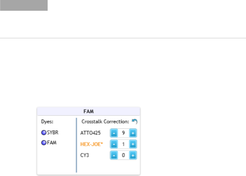
1 In the Supported Optical Configuration dialog box, locate the box for
the optical module that is or could be reporting crosstalk fluorescence
(i.e., the spillover optical module). The dyes that have the potential to
crosstalk with that optical module are listed in that box (e.g., the
HEX- JOE dye in the FAM optical module).
2 Change the crosstalk correction setting for the dye by adjusting the
value in the field.
The values in these fields are percentages of the total raw fluorescence.
They will be subtracted from the raw fluorescence signal for the optical
module when that dye is used as a target.
Crosstalk correction values that differ from the factory settings are
noted with an asterisk (*).
NOTE
The factory settings for crosstalk correction have been optimized to eliminate
potential crosstalk for dyes that are part of the default optical configuration.
Agilent does not recommend changing the crosstalk correction settings unless
you are using a new custom dye and the emission wavelength of that dye could be
detected by more than one optical module in the instrument.

2 Specifying Hardware and Software Settings
Change the default crosstalk correction settings
27 Agilent Aria Real-Time PCR Program
3 Click OK to apply your changes and close the dialog box.
To reset the crosstalk correction settings back to the factory settings:
1 In the Supported Optical Configuration dialog box, locate the box for
the optical module that you want to reset.
Crosstalk correction values that differ from the factory settings are
noted with an asterisk (*).
2 Within that box, click the reset icon next to Crosstalk Correction.
The crosstalk correction values for all dyes listed in the box are reset to
the factory values.
3 Click OK to apply your changes and close the dialog box.
NOTE
The Supported Optical Configuration dialog box does not include crosstalk
correction settings between the HEX-JOE and Cy3 optical modules because the
degree of crosstalk is too significant to be adequately corrected. Agilent does not
recommend using HEX-JOE and Cy3 together in a multiplex reaction.

Specifying Hardware and Software Settings 2
Set software preferences
Agilent Aria Real-Time PCR Program 28
Set software preferences
The Preferences dialog box is used for setting your preference on the
default file name configuration and for creating and selecting analysis
templates.
To open the Preferences dialog box: At the top of the program window,
click File > Preferences.
Set default file name configuration
To configure the default file name for experiments and projects:
1 In the Preferences dialog box, make sure File is selected at the top.
2 Next to New Experiment/Project File Naming, click one of the
following options:
•Default - Select this option to use the program's default file naming
system. For experiments, the default file name is “Experiment”
followed by the next available number (e.g., “Experiment 3"). For
projects, the default file name is “Project” followed by the next
available number (e.g., “Project 3").

2 Specifying Hardware and Software Settings
Set software preferences
29 Agilent Aria Real-Time PCR Program
•Custom - Select this option to configure your own file naming
system by selecting which pieces of information to include in the
default file name. Using the check boxes, you can select to include
the experiment type, the creation date for the experiment or project
(in format MM- DD- YYYY, DD- MM- YYYY, or YYYY- MM- DD), and the
time that the experiment or project was created.
3 Click OK to close the dialog box and save your changes.
Create and apply analysis templates
To create an analysis template that sets the default analysis settings for
experiments:
1 In the Preferences dialog box, select Defaults at the top.
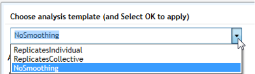
2 Type a name for the new template into the field below Choose analysis
template (and Select OK to apply).
Specifying Hardware and Software Settings 2
Set software preferences
Agilent Aria Real-Time PCR Program 30
3 Select when to apply the analysis template using the check boxes. You
can mark one check box, both check boxes, or neither check box.
• Mark Creating new experiment if you want to apply the analysis
template to all newly created experiments going forward.
• Mark Opening post run experiment if you want to apply the
analysis template anytime a post run experiment is opened in the
program.
• Clear both check boxes if you do not want the analysis template to
be automatically applied to experiments.
4 Click Add.
A message box opens asking you to confirm that you want to create the
new template. Click OK to continue.
5 Click OK to close the Preferences dialog box.
The program will apply the template to your experiments according to
the check box selections made in step 3.
Newly created analysis templates have only default analysis settings. See
“Configure and apply analysis templates” on page 192 for instructions
on configuring the analysis settings in the analysis template.
To select an existing analysis template to be applied to experiments:
1 In the Preferences dialog box, select Defaults at the top.
2 In the field below Choose analysis template (and Select OK to apply),
click the arrowhead to expand the drop- down list. The list contains all
of the existing analysis templates.
3 Select a template from the list.
4 Select when to apply the analysis template using the check boxes. You
can mark one check box, both check boxes, or neither check box.

2 Specifying Hardware and Software Settings
Set software preferences
31 Agilent Aria Real-Time PCR Program
• Mark Creating new experiment if you want to apply the analysis
template to all newly created experiments going forward.
• Mark Opening post run experiment if you want to apply the
analysis template anytime a post run experiment is opened in the
program.
• Clear both check boxes if you do not want the analysis template to
be automatically applied to experiments.
5 Click OK to close the Preferences dialog box. The program will apply
the template to your experiments according to the check box selections
made in step 3. See “Configure and apply analysis templates” on
page 192 for instructions on configuring the analysis settings in the
analysis template.
To delete an existing analysis template:
1 In the Preferences dialog box, select Defaults at the top.
2 In the field below Choose analysis template (and Select OK to apply),
click the arrowhead to expand the drop- down list. The list contains all
of the existing analysis templates.
3 Select a template from the list.
4 Click Delete.
5 In the message box that opens, click OK to confirm that you want to
delete the selected template.
6 If desired, select a different template from the list, or create a new
template.
7 When finished making changes, click OK to close the Preferences dialog
box.

Agilent Technologies
3
Performing Hardware and Software Tests and
HRM Calibrations
Run an instrument qualification test 33
Run the test 33
About the Qualification Test graphical data 34
Perform an Installation Qualification test 36
Run an HRM calibration plate (HCP) 38
Prepare the plate 38
Run an HCP 39
If the HCP fails 40
3 Performing Hardware and Software Tests and HRM Calibrations
Run an instrument qualification test
33 Agilent Aria Real-Time PCR Program
Run an instrument qualification test
Running a qualification test is one way to test for instrument errors. You
perform the test using a qualification test plate that must be purchased
separately from Agilent (part number 5190- 7708). The wells of the test
plate are pre- filled with the QPCR reagent mixture needed to run the test.
Run the test
Running a qualification test requires preparing the plate, running the
experiment on the AriaMx/AriaDx instrument, and checking the results.
To run a qualification test:
1 Prepare the qualification test plate according to the instructions that
came with the plate.
2 At the top of the program window, click Instrument > Qualification
Test.
A new tab opens for the Qualification Test experiment. The experiment
opens to the Thermal Profile screen.
3 Click Run.
The Instrument Explorer dialog box opens.
4 Locate the instrument that you will be using for the run and click Send
Config.
• If the instrument is not listed, see “Add instruments to your
network” on page 162 for instructions on searching for and adding
instruments.
• If this is the first time you have connected to an instrument since
last launching the Aria software, the Login dialog box opens. Select
your Username from the drop- down list, type your login password
into the Password field, and click Login. To log in with a different
user account, right- click on the instrument name and click Log off
current user. You can then log in using the desired user account
A message box opens notifying you that you must save the
experiment before you can connect to the instrument.
5 Click Save in the message box.
The Save As dialog box opens.
Performing Hardware and Software Tests and HRM Calibrations 3
Run an instrument qualification test
Agilent Aria Real-Time PCR Program 34
6 Select a folder for the experiment and type a name into the File name
field (or use the default). Click Save.
7 Take the prepared qualification test plate over to the instrument and
load it into the thermal block.
8 On the instrument touchscreen, open the primed experiment to the
Thermal Profile screen and press Run Experiment.
The instrument starts running the qualification test experiment.
9 Return to the PC program. The program directs you to the Raw Data
Plots screen, where you can monitor the progress of the run. See
“Monitor a run” on page 168.
10 At the end of the run, save the qualification test experiment to your PC
(see “Retrieve run data from the instrument” on page 173 for
instructions). Open the experiment in the Aria software on your PC.
11 Click Graphical Displays in the Experiment Area panel on the left side
of the screen. (See “About the Qualification Test graphical data” on
page 34 for more information about the graphs on this screen.)
12 Check the panel on the right side of the screen to determine if the
qualification test passed.
• If it passed, the panel displays Results Pass.
• If it failed, the panel displays Results Check.
If your qualification test failed, contact Agilent Technical Support for help
with troubleshooting. See “Contact Agilent Technical Support”.
About the Qualification Test graphical data
For a qualification test, the Graphical Displays screen includes graphs for
the Amplification Plots, the Standard Curve, and the Population
Distribution.
The Population Distribution graph is unique to Qualification Test
experiments. For each row of Unknown wells on the plate, this graph plots
the number of initial template copies calculated for that row against the
plate's column number. Because all wells in rows A, B, and C are
replicates and all wells in rows F, G, and H are replicates, the distribution
of the plot lines indicate the variability in initial template calculations
across the thermal block within the two populations (the ABC population
and the FGH population). In order to pass the qualification test, the

3 Performing Hardware and Software Tests and HRM Calibrations
Run an instrument qualification test
35 Agilent Aria Real-Time PCR Program
program requires that both populations be at least 98.5% distinct after
outlier wells are culled. The percent distinct for the Population
Distribution graph is displayed in the panel on the right side of the
Graphical Displays screen (next to % Distinct). Note that outlier wells are
plotted on the Population Distribution graph with a red x.
If your qualification test failed, Agilent's Technical Support staff may use
the graphical data to help troubleshoot the cause of the failure.

Performing Hardware and Software Tests and HRM Calibrations 3
Perform an Installation Qualification test
Agilent Aria Real-Time PCR Program 36
Perform an Installation Qualification test
You can run an Installation Qualification (IQ) test to determine if the Aria
software is properly installed on your system. The IQ test is comprised of
three separate tests:
• GUI Software Installation Qualification: Verifies the integrity of the
files and folders that are created as part of Aria software installation
• Permissions test: Verifies that the current user has full access to the
software's default file path for experiment files
• Connectivity test: Tests the communication between software and
instrument via FTP or TCP protocol service (if the firmware version is
determined to be outdated, a message box opens prompting you to
upgrade the firmware)
To perform the IQ test:
1 Click File > Qualifications. The Qualifications dialog box opens.

3 Performing Hardware and Software Tests and HRM Calibrations
Perform an Installation Qualification test
37 Agilent Aria Real-Time PCR Program
2 Next to Report is the file path and file name of the report that the
program generates at the end of the test. To select a different folder or
file name for the report, click Change. Then, in the Save As dialog box,
select a different folder and/or file name.
3 Click Start to start the test.
The program displays the status of the test in the Test Log area of the
dialog box. When finished, the program updates the Status column in
the dialog box and displays the overall result (Passed or Failed). If the
test failed, contact Agilent Technical Support for assistance.
4 Click Open Report to open the PDF report generated by the program.
5 To run the test again, click Reset to clear the results of the previous
test.
NOTE
The Operational option on the Qualifications dialog box has tools to run an
Operational Qualification (OQ) test. However, the Operational option is only
available to Agilent Service Engineers with an appropriate password.

Performing Hardware and Software Tests and HRM Calibrations 3
Run an HRM calibration plate (HCP)
Agilent Aria Real-Time PCR Program 38
Run an HRM calibration plate (HCP)
For experiments that include a high resolution melt (HRM) segment, before
you can analyze the HRM data on a Difference Plots graph, you must
associate the experiment with an HRM calibration plate (HCP) that was
run on the same instrument. The purpose of the HCP is to calculate an
offset temperature for each well in order to help normalize well- to- well
temperature variations. See “About HRM calibration plates” on page 67 for
more information.
Prepare the plate
Use the Agilent HRM Calibration Plate
Agilent offers a HRM Calibration Plate that you can use for HRM
calibration (Agilent part number 5190- 7701). The plate comes
pre- aliquoted with a master mix containing EvaGreen dye. See the plate's
user manual for more information.
Visit www.agilent.com/genomics for ordering information on the HRM
Calibration Plate.
Prepare the plate with your own reagents
Alternatively, you can prepare your own reagent mixture to be used in the
HCP run.
The 1x mixture needs to contain a purified amplicon at a concentration of
0.1- 0.3 mM. Ideally, the amplicon has a melting temperature (Tm) close to
that of the amplicon that you will be analyzing in your Allele
Discrimination experiment. The 1x mixture also needs to contain the same
DNA binding dye, at the same concentration, that you use in the QPCR
reactions for the Allele Discrimination experiment.
NOTE
A separate HRM software license is required in order to associate an experiment
with an HCP. To purchase a software license, contact your Agilent Sales
representative. The HRM license option is only available for the AriaMx system.
The license is not supported for the AriaDx system.
3 Performing Hardware and Software Tests and HRM Calibrations
Run an HRM calibration plate (HCP)
39 Agilent Aria Real-Time PCR Program
Instead of using a purified amplicon in your reagent mixture, you can use
a template, primers, and polymerase to produce the amplicon during the
HCP run. If you choose this approach, you need to add an amplification
segment to the default HCP thermal profile.
Note that the Aria calibration algorithms were tested and optimized using
the Agilent HRM Calibration Plate. Using your own HCP reagent mixture
may impact results.
Run an HCP
All HCP experiments must be set up and run directly from the instrument
(you cannot set up an HCP experiment from the Aria program on your
PC).
To run an HCP experiment:
1 On the instrument Home screen, press the HRM Calibration icon.
2 On the subsequent screen, press Open Default Experiment.
The default HCP experiment opens to the Plate Setup screen. All wells
are set to the Unknown well type and the SYBR dye is selected for
target detection in all wells
The EvaGreen dye used in the Agilent HCP kit is detectable with the
FAM/SYBR optic module.
3 Navigate to the Thermal Profile screen and press Run Experiment.
A message box opens on the touchscreen prompting you to save the
experiment. Press OK in the message box to save the experiment to the
HCP folder.
4 Select a file name for the experiment and press Save.
The instrument starts running the experiment.
5 After the run, a message box opens on the screen notifying you if the
HCP passed or failed.
• If it passed, copy the post- run HCP experiment file to your PC (see
“Retrieve run data from the instrument” on page 173 for
instructions). You can then use the HCP to calibrate HRM data from
an experiment. See “Assign an HRM calibration plate” on page 183
for instructions.

Performing Hardware and Software Tests and HRM Calibrations 3
Run an HRM calibration plate (HCP)
Agilent Aria Real-Time PCR Program 40
• If it failed, you cannot use the HCP to calibrate HRM data from an
experiment. See “If the HCP fails”, below, for information on failed
HCPs.
If the HCP fails
If the HCP fails the system's quality check, the touchscreen displays a
message box at the end of the HCP run notifying you of the failure. You
will also see a warning icon (as shown below) if you open the experiment
in the Aria program on your PC.
Possible causes of a failed plate include pipetting errors during set up of
the plate and amplicon degradation. If you find your HCP runs repeatedly
fail, try setting up the plate using the Agilent HRM Calibration Plate. If
problems persist, contact Agilent Technical Support (see “Contact Agilent
Technical Support” on page 370). Note that you cannot associate a failed
HCP with an experiment.
3 Performing Hardware and Software Tests and HRM Calibrations
Run an HRM calibration plate (HCP)
41 Agilent Aria Real-Time PCR Program

Agilent Technologies
4
Creating/Opening an Experiment
Overview of the Getting Started screen 43
Tools available on the Getting Started screen 44
About the Aria file types 45
Quick Start Protocol 46
How to create, set up, run, analyze, and generate reports for an
experiment 46
Create a new experiment 49
Create an experiment based on experiment type 49
Create an experiment from a template 50
Create an experiment from a LIMS data file 51
Open an existing experiment 53
Save a copy of an existing experiment 54
Create a template from an existing experiment 55
Convert an experiment to a new experiment type 56

4 Creating/Opening an Experiment
Overview of the Getting Started screen
43 Agilent Aria Real-Time PCR Program
Overview of the Getting Started screen
The tools on the Getting Started screen allow you to create a new
experiment (from scratch or from a template), create a new multiple
experiment analysis project, or open an existing experiment or project.
To open the Getting Started screen: At the top of the program window,
click File > New. Alternatively, click the icon to open a new tab in the
program. The new tab opens to the Getting Started screen.

Creating/Opening an Experiment 4
Overview of the Getting Started screen
Agilent Aria Real-Time PCR Program 44
Tools available on the Getting Started screen
The content in the center of the screen changes depending on which
option is selected in the panel on the left. These options are described in
the table below
Option Description
New Experiment
Experiment Types Click this option to create a new experiment based on the desired experiment type.
The center of the screen displays the experiment types for selection.
My Templates Click this option to create a new experiment from a template. The center of the
screen displays the template files in the Experiments Templates folder that is
created during program installation.
From LIMS file... Click this option to create a new experiment from a LIMS data file that specifies the
plate setup and, optionally, the thermal profile. The center of the screen displays the
Import From LIMS Data File wizard.
New Project
Multiple Experiment
Analysis
Click this option to create a new project for analyzing and comparing multiple
post-run experiments. The center of the screen displays tools for adding
experiments to the new project.
Saved
Recently Opened Click this option to open an existing experiment or project that you recently
accessed. The center of the screen displays a list of experiments that you have
recently opened.
Browse Click this option to open an existing experiment or project by browsing to a desired
folder.
Links at the bottom of the screen
License Click this link to open a message box about licensing. In the message box, click
License Agreement to view the full text of the Aria software license agreement.
© Agilent Technologies Click this link to open the About message box. This box displays the full version
number of the software.
Contact Support Click this link to create a new email message directed to the Agilent Technical
Support group.
4 Creating/Opening an Experiment
Overview of the Getting Started screen
45 Agilent Aria Real-Time PCR Program
About the Aria file types
Three different files types can be created in the Aria program: an
experiment file, a protocol template file, and a project file. These file types
are summarized below.
Experiment Files (*.amxd or *.adxd)
In the Aria software, experiments of all types (Quantitative PCR,
Comparative Quantitation, Allele Discrimination, and User Defined) are
saved as experiment files. When an experiment file is open, the program
includes screens for defining the wells of the experimental plate, setting
up the thermal profile, running the experiment, and analyzing the results
of that run. AriaMx experiment files are given the extension amxd, and
AriaDx experiment files are given the extension adxd.
Template Files (*.amxt or *.adxt)
In addition to saving an experiment as an experiment file, the plate setup
and thermal profile of an experiment can be saved as a template file.
Creating a new experiment from a template file allows you to quickly set
up new experiments that require a similar plate setup or thermal profile.
AriaMx template files are given the extension amxt, and AriaDx template
files are given the extension adxt.
Project Files (*.amxp or *.adxp)
Multiple experiment analysis projects are saved as project files. Up to 8
post- run experiment files (of the same experiment type) can be added to
a project, enabling you to analyze the results side by side or combine
results across experiments. AriaMx project files are given the extension
amxp, and AriaDx project files are given the extension adxp.
Creating/Opening an Experiment 4
Quick Start Protocol
Agilent Aria Real-Time PCR Program 46
Quick Start Protocol
How to create, set up, run, analyze, and generate reports for an experiment
1. Create the experiment
• Open a new tab. On the Getting Started screen, under New
Experiment, click Experiment Types (to create a new experiment by
the experiment type) or My Templates (to create a new experiment
from a template).
2. Set up the plate
• After creating the experiment, the experiment opens to the Plate
Setup screen.
• Assign the plate properties based on experiment type, including
assigning well types, replicate numbers, and dyes/targets. See the
topics below for instructions specific to each experiment type.
“Assign plate properties for a Quantitative PCR DNA Binding Dye
experiment” on page 86
“Assign plate properties for a Quantitative PCR Fluorescence Probe
experiment” on page 94
“Assign plate properties for a Comparative Quantitation experiment”
on page 102
“Assign plate properties for an Allele Discrimination DNA Binding
Dye experiment” on page 113
“Assign plate properties for an Allele Discrimination Fluorescence
Probe experiment” on page 122
“Assign plate properties for a User Defined experiment” on page 131
3. Set up the thermal profile
• Navigate to the Thermal Profile screen. (Click Thermal Profile in the
Experiment Area panel on the left side of the screen.)
• Edit the thermal profile as desired, or use the default/template
thermal profile.
4 Creating/Opening an Experiment
Quick Start Protocol
47 Agilent Aria Real-Time PCR Program
4. Run the experiment
• From the Thermal Profile screen, click Run. In the Instrument
Explorer dialog box that opens, locate the instrument and click Send
Config.
• Load your reaction plate into the instrument's thermal block. On the
instrument touchscreen, open the primed experiment to the Thermal
Profile screen and press Run.
• If desired, monitor the progress of the run from your PC.
5. Set the analysis criteria
• When the run is finished, navigate to the Analysis Criteria screen.
(Click Analysis Criteria in the Experiment Area panel on the left
side of the screen.)
• Select the wells, well types, and targets to include in the analysis,
specify the treatment of replicate wells, and select the data collection
marker to use for analysis. If your experiment included a high
resolution melt segment (HRM), assign an HRM calibration plate to
the experiment.
6. Analyze the data
• Navigate to the Graphical Displays screen. (Click Graphical Displays
in the Experiment Area panel on the left side of the screen.)
• View the results of the analysis and customize analysis settings for
individual graphs. See the topics below for instructions specific to
each graph.
“View the Amplification Plots” on page 197
“View the Melt Curve - Raw/Derivative Curve” on page 212
“View the Melt Curve - Difference Plots” on page 218
“View the Standard Curve” on page 225
“View the Relative Quantity” on page 230
“View the Allele Determination graph” on page 235
Creating/Opening an Experiment 4
Quick Start Protocol
Agilent Aria Real-Time PCR Program 48
7. Export the results
• To generate a report of the results, navigate to the Generate Report
screen (click Generate Report in the Experiment Area panel on the
left side of the screen). Configure and create the report according to
your selections.
• To export numerical data from the experiment, navigate to the
Export Data screen (click Export Data in the Experiment Area panel
on the left side of the screen). Select the file type and information
you want to export.

4 Creating/Opening an Experiment
Create a new experiment
49 Agilent Aria Real-Time PCR Program
Create a new experiment
The Getting Started screen allows you to create a new experiment. To
create the new experiment from scratch, you start by selecting the
experiment type. To create the new experiment from a template or LIMS
data file, you start by selecting the template or LIMS data file that you
want to use. Once created, you can edit the plate setup and thermal
profile for the new experiment.
To open the Getting Started screen: At the top of the program window,
click File > New, or click the icon, to open a new tab in the program.
The new tab opens to the Getting Started screen.
Create an experiment based on experiment type
When you create a new experiment based on experiment type, your
selection of the experiment type determines some of the setup options and
analysis outputs. The thermal profile of the new experiment is set to the
default for the chosen experiment type. The plate setup of the experiment
is blank, but the available well types and other well configuration tools on
the Plate Setup screen are specific to the experiment type.
To create an experiment based on experiment type:
1 Open the Getting Started screen.
2 Under New Experiment, click Experiment Types.
The center of the screen displays all the available experiment types. See
“Overview of Experiment Types” on page 59.
3 Click the desired experiment type to select it.
4 In the Experiment Name field, type a name for the new experiment,
then click Create.
The program creates the new experiment and opens the experiment to
the Plate Setup screen.
NOTE
At step 3, you can double-click the desired experiment type to select it with the
default experiment name. The program creates the new experiment and opens the
experiment to the Plate Setup screen (or to the Thermal Profile screen for User
Defined experiments).

Creating/Opening an Experiment 4
Create an experiment from a template
Agilent Aria Real-Time PCR Program 50
Create an experiment from a template
When you create a new experiment from a template, the experiment has
the plate setup and thermal profile of the selected template. After you
create the experiment, you can edit the plate setup and thermal profile as
desired.
The Aria software comes with three sample template files. The templates
are available in the folder C:\Users\Public\Public Documents\Agilent
Aria\Experiment Templates.
To create an experiment from a template:
1 Open the Getting Started screen.
2 Under New Experiment, click My Templates.
The center of the screen displays the template files in the default
template folder.
3 In the Experiment Name field, type a name for the new experiment.
4 Select the desired template and create the experiment.
• If the template is in the default folder, click directly on the template
to select it and then click Create (or double- click directly on the
template). The program creates the new experiment and opens the
experiment to the Plate Setup screen.
• If the template is not in the currently selected folder, click the
Browse to Template icon (shown below) to open the browser window.
Browse to the folder of the desired template file. Select the file and
click Open. The program creates the new experiment and opens the
experiment to the Plate Setup screen.
NOTE
You can toggle between displaying the templates in list format and tile format by
clicking the icons in top right corner.
= List view icon
= Tile view icon
4 Creating/Opening an Experiment
Create an experiment from a template
51 Agilent Aria Real-Time PCR Program
Create an experiment from a LIMS data file
To create a new experiment from a LIMS data file, you must provide a
valid file. The file may be generated by exporting a post- run Aria
experiment to a LIMS data file (see “Export to a LIMS data file” on
page 262), by setting up a text file in the necessary Aria- supported LIMS
data file format, or by a LIMS software program. See “LIMS File Format
for Aria Software” on page 361 for information on format requirements for
LIMS data files used to create new experiments in the Aria program. After
you import the file and create the experiment, you can edit the plate
setup and thermal profile as desired from the Plate Setup and Thermal
Profile screens.
The Aria software comes with sample LIMS data files (text files and CSV
files). The files are available in the folder C:\Users\Public\Public
Documents\Agilent Aria\Sample LIMS Import Files.
To create an experiment from a LIMS data file:
1 Open the Getting Started screen.
2 Under New Experiment, click From LIMS file....
The center of the screen displays the Import From LIMS Data File
wizard.
3 In the Filename field under LIMS data file, type the file path for the
LIMS data file, or click Browse to browse to and select the LIMS data
file. The file type can be a text file (*.txt) or a CSV file (*.csv).
The program populates the fields in the Experiment setup and
Thermal profile setup areas of the LIMS Data File wizard using the
available information from the selected file. Note that the file may not
include all experiment details.
4 (Optional) Edit the information in the Experiment setup fields as
desired.
• In the Name field, type a name for the experiment. If the imported
LIMS data file specified the experiment name, then the field is
populated with that name.
• In the Type drop- down list, select an experiment type. If the
imported LIMS data file specified the experiment type, then the
drop- down list is set to that selection. See “Overview of Experiment
Types” on page 59 for descriptions of the Aria experiment type
options.
Creating/Opening an Experiment 4
Create an experiment from a template
Agilent Aria Real-Time PCR Program 52
• In the Notes field, type any experiment notes that you want
associated with the new experiment. If the imported LIMS data file
included experiment notes, then the field is populated with those
notes.
5 Click Next.
The screen displays the plate setup information for the experiment.
6 (Optional) Edit the Reference Dye selection and other target information
as permitted for the experiment type.
7 Click Finish.
The program creates the new experiment and opens the experiment to
the Plate Setup screen. A message box opens confirming that the
experiment has been successfully imported. Click OK to close the
message box.

4 Creating/Opening an Experiment
Open an existing experiment
53 Agilent Aria Real-Time PCR Program
Open an existing experiment
The program allows you to open up to 5 experiments at a time, or one
project at a time. The program displays each open experiment or project
on its own tab.
To open an experiment in a new tab:
1 Click the icon to the right of the tabs to open a new tab.
The new tab opens to the Getting Started screen.
2 Click one of the options under Saved:
• To open an existing experiment that you recently accessed, click
Recently Opened. The center of the screen displays a list of
experiments and projects that you have recently opened. Double- click
the experiment you want to open. The program opens the experiment
to the Plate Setup screen.
• To browse to the folder of the experiment, click Browse. The Open
dialog box opens. Browse to the folder location of the experiment.
Select the experiment and click Open. The dialog box closes and the
program opens the experiment to the Plate Setup screen.
To open an experiment in an already open tab:
1 From the toolbar, click File > Open.
The Open dialog box opens. If an experiment or project is currently
open in the tab, the program closes that experiment or project, and
prompts you to save any changes.
2 Browse to the folder location of the experiment. Select the experiment
and click Open.
The dialog box closes and the program opens the experiment to the
Plate Setup screen.
Creating/Opening an Experiment 4
Save a copy of an existing experiment
Agilent Aria Real-Time PCR Program 54
Save a copy of an existing experiment
You can use the Save As command to copy the open experiment and save
it with a new experiment name.
To copy an existing experiment using the Save As command:
1 Open the existing experiment that you want to copy.
2 Click File > Save As.
The Save As dialog box opens.
3 Select a folder for the new experiment and type a name into the file
name field.
4 Click Save.
The program saves the open experiment under the new name.
4 Creating/Opening an Experiment
Create a template from an existing experiment
55 Agilent Aria Real-Time PCR Program
Create a template from an existing experiment
You can use the Save As Template command to create a template file
based on the plate setup and thermal profile of an existing experiment.
You can later use the template to quickly create new experiments. See
“Create an experiment from a template” on page 50.
To create a template from an existing experiment using the Save As
Template command:
1 Open the existing experiment that you want to create a template from.
2 Click File > Save As Template.
The Save As dialog box opens. If you are running the AriaMx mode of
the software, the file type set to AriaMx Template Files (*.amxt). If
you are running the AriaDx mode of the software, the file type set to
AriaDx Template Files (*.adxt).
3 Select a folder for the new template and type a name into the file name
field.
4 Click Save.
The dialog box closes and the program saves the new template file
(*.amxt or *.adxt) to the designated folder.
Creating/Opening an Experiment 4
Convert an experiment to a new experiment type
Agilent Aria Real-Time PCR Program 56
Convert an experiment to a new experiment type
The Convert Experiment Type command can convert a post- run
experiment into another experiment type. This command is useful when
the experiment was set up as one type and the data needs to be
re- analyzed as a different experiment type. The program applies the
analysis algorithms and display options based on the new experiment type.
To convert an experiment to a new experiment type:
1 Open the existing post- run experiment that you want to convert.
2 Click File > Convert Experiment Type, and in the sub- menu, select the
new experiment type.
A message box opens notifying you that the conversion was successful
and that some well types may have changed.
3 Click OK to close the message box.
The program creates a new experiment file for the converted
experiment and opens the experiment to the Plate Setup screen. By
default, the new experiment has the same name as the parent
experiment with the word “Converted” added at the beginning.
4 Click File > Save As.
The Save As dialog box opens.
5 Select a folder for the new experiment. Type a name into the file name
field or use the default file name.
6 Click Save.
The program saves the new experiment to the designated folder.
4 Creating/Opening an Experiment
Convert an experiment to a new experiment type
57 Agilent Aria Real-Time PCR Program

Agilent Technologies
5
Selecting an Experiment Type
Overview of Experiment Types 59
Quantitative PCR 59
Comparative Quantitation 59
Allele Discrimination - Fluorescence Probes 60
Allele Discrimination - DNA Binding Dye with High-Resolution
Melt 60
User Defined 60
The Quantitative PCR Experiment Type 61
Multiplexing quantitative PCR experiments 61
Well types for Quantitative PCR experiments 62
The Comparative Quantitation Experiment Type 63
Normalizing chance variations in target levels 63
Determining amplification efficiencies for the targets of interest and
normalizer targets 64
Including biological replicates in comparative quantitation 65
Well types for Comparative Quantitation experiments 66
The Allele Discrimination - DNA Binding Dye Experiment Type 67
About HRM calibration plates 67
Well types for Allele Discrimination - DNA Binding Dye
experiments 68
The Allele Discrimination - Fluorescence Probe Experiment Type 69
Well types for Allele Discrimination - Fluorescence Probe
experiments 70
The User Defined Experiment Type 71
5 Selecting an Experiment Type
Overview of Experiment Types
59 Agilent Aria Real-Time PCR Program
Overview of Experiment Types
The Aria program offers a variety of experiment types. Each experiment
type was designed for a specific application and has its own unique
options for experimental setup and analysis that are specialized for that
application. The Aria experiment types are summarized below.
Quantitative PCR
The Quantitative PCR experiment type is the best choice when you need
to determine the exact quantity of a particular DNA target in the
experimental template samples. This experiment type uses a standard
curve produced with samples of known template quantity to derive the
initial quantity of the target in the experimental sample.For more
information, see “The Quantitative PCR Experiment Type” on page 61.
The program offers two sub- types for the Quantitative PCR experiment
type: DNA Binding Dye Including Standard Melt and Fluorescence Probe.
These sub- types differ by the type of chemistry used to detect the PCR
products. In the DNA Binding Dye Including Standard Melt sub- type,
detection is based on signal from a double- stranded DNA binding dye, e.g.,
SYBR Green, and the default thermal profile includes a melt curve. In the
Fluorescence Probe sub- type, a target- specific probe, e.g., a TaqMan probe,
is used for target detection.
Comparative Quantitation
The Comparative Quantitation experiment type is best used for comparing
levels of RNA or DNA across samples when you do not require
information about the absolute amount of target. Most common is the
comparison of amounts of mRNA in treated versus untreated, or normal
versus diseased cells or tissues. The program will ask you to identify
which wells contain the control sample (called the “calibrator”) and which
wells contain the associated experimental sample (called the “unknown”).
For accurate results, you need to normalize the data to the quantity of a
target gene (called a “normalizer”) that is known to be unaffected by the
experimental conditions, such as a housekeeping gene. For more
information, see “The Comparative Quantitation Experiment Type” on
page 63.
Selecting an Experiment Type 5
Overview of Experiment Types
Agilent Aria Real-Time PCR Program 60
Allele Discrimination - Fluorescence Probes
The Allele Discrimination experiment type is used to discriminate between
two alleles in a DNA sample. For more information, see “The Allele
Discrimination - Fluorescence Probe Experiment Type” on page 69.
The program offers two sub- types for the Allele Discrimination experiment
type. In the sub- type Fluorescence Probe, you use two fluorogenic probes
labeled with different dyes to discriminate between two alleles in a DNA
sample. For example, if amplification in an unknown DNA sample is
detected for the dye identifying the wild- type allele but not for the dye
identifying a mutant allele, the sample can be designated as wild- type
homozygous.
Allele Discrimination - DNA Binding Dye with High-Resolution Melt
The Allele Discrimination experiment type is used to discriminate between
two alleles in a DNA sample. For more information, see “The Allele
Discrimination - DNA Binding Dye Experiment Type” on page 67.
The program offers two sub- types for the Allele Discrimination experiment
type. In the sub- type Fluorescence Probe, you use two fluorogenic probes
labeled with different dyes to discriminate between two alleles in a DNA
sample. For example, if amplification in an unknown DNA sample is
detected for the dye identifying the wild- type allele but not for the dye
identifying a mutant allele, the sample can be designated as wild- type
homozygous
User Defined
The User Defined experiment type provides the greatest flexibility in setup
and analysis of an experiment. All the well types and other plate setup
options that are available across the other experiment types are available
on the Plate Setup screen in a User Defined experiment. Similarly, on the
Thermal Profile screen, you can add any type of segment to the thermal
profile, and on the Graphical Displays screen, you can view the results for
any of the experiment type- specific graphs.
5 Selecting an Experiment Type
The Quantitative PCR Experiment Type
61 Agilent Aria Real-Time PCR Program
The Quantitative PCR Experiment Type
In Quantitative PCR experiments, the instrument detects the fluorescence
of one or more dyes or fluorophores during each cycle of the thermal
cycling process and a fluorescence value is reported for each
dye/fluorophore at each cycle. Generally, you want the instrument to
acquire fluorescence readings during the annealing stage of thermal
cycling.
You can quantify the initial copy numbers of RNA or DNA targets based
on quantification cycle (Cq) determinations. The Cq is defined as the cycle
at which a statistically- significant increase in fluorescence is first
detected. The threshold cycle is inversely proportional to the log of the
initial copy number. In other words, the more template that is present
initially, the fewer the number of cycles required for the fluorescence
signal to be detectable above background. The Aria program offers both
automatic and manual methods for determination of the threshold
fluorescence level that is used to determine Cq values.
Typical Quantitative PCR experiments use a standard curve to quantitate
the amount of target present in an experimental sample (called the
“unknown” sample since the quantity of the target is unknown). In this
method, you set up the plate to amplify a series of standards to generate
a standard curve that relates initial template quantity to Cq. You generate
the standards by serial dilution of a template sample that contains a
known quantity of the target under investigation. The program then uses
the standard curve to derive the initial template quantity of this target in
the unknown samples based on their Cq values.
Multiplexing quantitative PCR experiments
The instrument records fluorescence readings for each sample on all five
optical modules. This allows you to use multiplex PCR for quantitation of
multiple targets in the same well by using spectrally- distinct dyes to
detect each target. The Aria program reports each target in each well
separately on amplification plots and other graphical results displays.

Selecting an Experiment Type 5
The Quantitative PCR Experiment Type
Agilent Aria Real-Time PCR Program 62
Well types for Quantitative PCR experiments
Well Type Description
Unknown Contains a complete reaction mixture including a test template that
contains an unknown amount of the target-of-interest.
Buffer Contains only buffer; used to monitor the background fluorescence
attributable to the buffer.
NAC No amplification control; contains all reaction components except DNA
polymerase.
NTC No template control; contains all reaction components except the
template nucleic acid.
This well type is useful for detecting amplicon contamination.
Standard Contains a complete reaction mixture including a known concentration
of the target-of-interest.
This well type is used to generate a standard curve, which is then used to
relate the quantification cycle (Cq) to initial template quantity in
Unknown wells and calculate the amplification efficiency.
No RT No reverse transcriptase control; contains all QRT-PCR reaction
components except reverse transcriptase.
In one-step RT-PCR assays, this control is useful for assessing levels of
genomic DNA carryover that may contribute to fluorescence increase in
the sample.
5 Selecting an Experiment Type
The Comparative Quantitation Experiment Type
63 Agilent Aria Real-Time PCR Program
The Comparative Quantitation Experiment Type
The Comparative Quantitation experiment type provides an efficient
method for comparing levels of RNA or DNA across samples when you do
not require information about the absolute amount of target in any
sample. The most common application is the comparison of amounts of
mRNA in treated versus untreated, or normal versus diseased cells or
tissues.
For many gene expression studies, your experiments do not require you to
determine the absolute amount of a target in a particular sample; evidence
of a relative increase or decrease in expression, compared to a sample of
reference, is sufficient. The sample of reference is referred to as the
calibrator. For example, in a study in which a large number of compounds
are screened for the ability to induce the expression of a certain set of
genes in HeLa cells, the calibrator might be a nucleic acid sample isolated
from an untreated HeLa cell culture. In a study involving the expression
of a cancer marker gene, the calibrator might be a nucleic acid sample
isolated from the normal, non- diseased part of the organ, whereas the test
samples (referred to in the program as Unknowns) are nucleic acids
isolated from the diseased tissue of the same patient. The expression level
of the target- of- interest (i.e., the gene you are studying) in the calibrator
is defined as 1× (or 1.0). Expression levels in all unknown samples are
reported as a fold difference relative to this calibrator benchmark.
Normalizing chance variations in target levels
The quantity of a target- of- interest present across a set of
independently- isolated samples is subject to many variables such as
sample- to- sample differences in total amount of input nucleic acid and
differences in the efficiency of RNA extraction or reverse transcription.
You can include a normalizer target in the assay to reduce the effect of
these spurious variations that do not reflect true differences in target
abundance as a result of experimental treatment. Any gene with little to
no variance in expression due to the experimental treatment can serve as
a normalizer. (Commonly- used examples include housekeeping genes such
as GAPDH, cyclophilin, GUS, TFIID, or 18S, or 28S ribosomal RNA.) The
abundance of the normalizer and the target- of- interest should be similar.
In a typical Comparative Quantitation experiment, you would set up the
wells containing the calibrator sample to run alongside a variety of
Selecting an Experiment Type 5
The Comparative Quantitation Experiment Type
Agilent Aria Real-Time PCR Program 64
unknown samples to test the effect of some variable on the expression
level of one or more genes of interest. You can set up the reactions
amplify the normalizer target in the same well as the target- of- interest
(using multiplexing) or set up the reactions to amplify the normalizer and
the target- of- interest in different wells.
During analysis, the program automatically adjusts the levels of the
target- of- interest in both Unknown and Calibrator wells to compensate for
differences in the levels of the normalizer. The program then compares the
normalized value for each unknown sample to the normalized calibrator
value, and reports the relative quantity for each unknown. (The expression
level of the target- of- interest in the Calibrator wells is set to 1.0.)
Establish the amplification efficiencies of the normalizer target and the
target- of- interest before you use a particular normalizer in a Comparative
Quantitation experiment.
See the following section (“Determining amplification efficiencies for the
targets of interest and normalizer targets”) for more information.
Determining amplification efficiencies for the targets of interest and
normalizer targets
In developing a Comparative Quantitation experiment, it is important that
the amplification efficiencies of the target- of- interest and the normalizer
target are reproducible and, ideally, very similar. To measure the
amplification efficiency for each target, generate a standard curve in a
Quantitative PCR experiment. When running a standard curve for the sole
purpose of determining the amplification efficiency for a particular target,
it is not necessary to know the exact quantity of your targets. Instead, you
can use serially diluted template as the standard samples and assign the
standard quantities in Plate Setup using the “relative” unit designation.
The program then analyzes the standard curve data and calculates the
amplification efficiency from the slope of the curve. (See “View the
R- squared values, slopes, and amplification efficiencies” on page 227 for
more information on deriving amplification efficiencies from standard
curves.)
If differences in amplification efficiency exist
In an idealized Comparative Quantitation experiment, the amplification
efficiencies for the target- of- interest and normalizer target must be
5 Selecting an Experiment Type
The Comparative Quantitation Experiment Type
65 Agilent Aria Real-Time PCR Program
identical in order to allow a direct correction of target levels across
samples. However, if you find from your standard curves that the
target- of- interest and normalizer have different amplification efficiencies,
the program allows you to compensate for this difference using the
settings under Amplification Efficiencies in the Graphical Displays screen.
To access these settings, expand the menu in the panel on the right side
of the Graphic Displays screen. (See “Enter the amplification efficiencies
for the targets ” on page 233 for detailed instructions.)
Including biological replicates in comparative quantitation
In QPCR, biological replicates are template samples that were isolated
independently but from biologically- identical sources (sources that are
genetically identical are of the same cell type and were treated identically
during experimentation). For example, two samples of cDNA that were
isolated from the same tissue source in two different mice that were
exposed to identical conditions and have the same genotype would be
biological replicates. Biological replicates help you determine the level of
variability in gene expression for your specific experiment that is due to
uncontrolled biological variation from sample to sample.
When setting up the plate for a Comparative Quantitation experiment, you
may designate two or more samples as biological replicates while assigning
the sample names. Samples that are biological replicates are assigned the
same sample name but have different biological replicate ID numbers.
During analysis, the program treats biological replicates independently as
different samples.
If the experiment includes multiple biological replicates of the calibrator
sample, you can designate only one of the samples within the set of
replicates as the calibrator. You can change the assignment of the
calibrator after the run if you want to re- analyze the results using a
different calibrator designation.

Selecting an Experiment Type 5
The Comparative Quantitation Experiment Type
Agilent Aria Real-Time PCR Program 66
Well types for Comparative Quantitation experiments
Well Type Description
Unknown Contains a complete reaction mixture including a test template that
contains an unknown amount of the target-of-interest.
Calibrator Contains a complete reaction mixture including an unknown amount of
the target-of-interest.
The level of a target-of-interest in the calibrator wells is set to 1.0 for
comparison to the relative quantities in unknown samples.
NTC No template control; contains all reaction components except the
template nucleic acid.
Standard Contains a complete reaction mixture including a known concentration
of the target-of-interest.
This well type is used to generate a standard curve, which is then used to
relate the quantification cycle (Cq) to initial template quantity in
Unknown wells and calculate the amplification efficiency.
No RT No reverse transcriptase control; contains all QRT-PCR reaction
components except reverse transcriptase.
In one-step RT-PCR assays, this control is useful for assessing levels of
genomic DNA carryover that may contribute to fluorescence increase in
the sample.
NAC No amplification control; contains all reaction components except DNA
polymerase.
Buffer Contains only buffer; used to monitor the background fluorescence
attributable to the buffer.

5 Selecting an Experiment Type
The Allele Discrimination - DNA Binding Dye Experiment Type
67 Agilent Aria Real-Time PCR Program
The Allele Discrimination - DNA Binding Dye Experiment Type
The Allele Discrimination - DNA Binding Dye experiment type is used to
discriminate between two alleles of a gene in a genomic DNA or cDNA
sample using a double- stranded DNA binding dye, such as SYBR Green or
EvaGreen dye, and a high- resolution melt (HRM).
HRM analysis is a technique used for genotyping samples that include a
single nucleotide polymorphism (SNP) in the DNA sequence. Applications
that may use HRM analysis include species identification, mutation
screening, and haplotype characterization. When using the allele
discrimination experiment type for HRM analysis, you set up the
experiment to amplify all alleles in the same well using the same set of
primers, and the program detects all alleles using the same
double- stranded DNA- binding dye (such as SYBR Green or EvaGreen dye).
The thermal profile includes a melt segment so that melt curves of the
targets can be generated. Even DNA amplicons that differ in sequence by
only a single nucleotide will yield slightly different melt curves. An Allele
Discrimination experiment that uses HRM analysis needs to include
positive control samples for each base pair possibility at the SNP location
(homozygous as well as heterozygous positive control samples).
On the Graphical Displays screen, Difference Plots show the difference in
fluorescence between two plots during a melt ramp (Y axis) as a function
of temperature (X axis). By graphing the difference in fluorescence, the
program can detect even slight differences between two melt curves. You
can use the difference plots to compare samples of unknown genotype to
positive control samples, and visually determine which genotype group the
target in the unknown sample falls into.
About HRM calibration plates
During the HRM segment of the thermal profile, the instrument ramps the
temperature of the thermal block in 0.2°C increments. At any given target
temperature, very slight differences in the exact temperature may exist
from well to well across the thermal block. The purpose of an HRM
calibration plate (HCP) is to calculate an offset temperature for each well
NOTE
A separate HRM software license is required in order to view the Difference Plots.
To purchase a software license, contact your Agilent Sales representative.

Selecting an Experiment Type 5
The Allele Discrimination - DNA Binding Dye Experiment Type
Agilent Aria Real-Time PCR Program 68
in order to help normalize these temperature variations. The offset
temperature is the difference between the Tm (melting temperature) in
any given well and the average Tm for the plate. When you associate your
Allele Discrimination experiment with an HCP experiment, the program
subtracts the offset temperature from the calculated Tm in each well. This
normalization improves the accuracy and clarity of the difference plots
and the raw/derivative melt curves.
In order to calculate the offset temperatures, an HCP must contain the
identical amplicon in each well. During the HCP run, that amplicon is
melted in an HRM segment. The program then calculates a Tm for each
well and an average Tm for the plate.
All HCP experiments must be set up and run directly from the instrument
(you cannot set up an HCP experiment from your PC). See “Run an HRM
calibration plate (HCP)” on page 38 for instructions.
You can use the same HCP experiment for multiple Allele Discrimination
experiments. For each instrument, Agilent recommends running a new
HCP experiment at least once per year.
Well types for Allele Discrimination - DNA Binding Dye experiments
Well Type Description
Unknown Contains a complete reaction mixture including a test template that
contains an unknown amount of the specific target.
NTC No template control; contains all reaction components except the
template nucleic acid.
This control is useful for detecting amplicon contamination.
Homo Allele A Contains a complete reaction mixture with a positive control template
that is known to be homozygous for allele A.
Home Allele B Contains a complete reaction mixture with a positive control template
that is known to be homozygous for allele B.
Hetero Contains a complete reaction mixture with a heterozygous positive
control template that is known to include both allele A and allele B.
5 Selecting an Experiment Type
The Allele Discrimination - Fluorescence Probe Experiment Type
69 Agilent Aria Real-Time PCR Program
The Allele Discrimination - Fluorescence Probe Experiment Type
The Allele Discrimination experiment type is used to discriminate between
two alleles of a gene in a genomic DNA or cDNA sample. An Allele
Discrimination experiment can be performed two different ways: using
fluorescent probes (as described below) or using a double- stranded DNA
binding dye.
Using the probe method for allele discrimination, two fluorescent probes
labeled with two spectrally distinct dyes are used to discriminate between
the two alleles and, subsequently, determine the genotype of a sample. For
example, if the program detects amplification in an unknown DNA sample
for the dye identifying the wild- type allele but not for the dye identifying
a mutant allele, the program designates the sample as wild- type
homozygous. If the program detects amplification in an unknown DNA
sample for the dye identifying the mutant allele but not for the dye
identifying the wild- type allele, the program designates the sample as
mutant homozygous. If the program detects amplification for both dyes, it
designates the unknown sample as heterozygous for the two alleles. With
properly designed probes, this assay is sensitive enough to detect a
single- base difference (single nucleotide polymorphism or SNP) between
two alleles.
The program uses the quantification cycle (Cq) value for each target in
each sample to determine the genotypes of the samples. A Cq value of 24
to 32 is expected for a sample that contains the specific allele recognized
by the probe. A Cq value equal to the final cycle of the PCR reaction
(typically 40) or equal to the Cq of the negative control samples indicates
the absence of a specific allele. The program displays the results in the
Allele Determination graph, which is a scatter plot that shows the Cq for
the dye specific to one allele plotted against the Cq for the dye specific to
the other allele. The program groups plotted points according to their
positions on the graph, providing a convenient visualization of samples
which share the same genotype (allelic composition).
In the analysis of real- time Allele Discrimination experiments that use
fluorescence probes (e.g., TaqMan probes), you would typically monitor
and report fluorescence at the end of the annealing/extension step. At
that point, the polymerase has already extended across the template and
hydrolyzed any probe that had annealed.

Selecting an Experiment Type 5
The Allele Discrimination - Fluorescence Probe Experiment Type
Agilent Aria Real-Time PCR Program 70
Well types for Allele Discrimination - Fluorescence Probe experiments
Well Type Description
Unknown Contains a complete reaction mixture including a test template that
contains an unknown amount of the specific target.
NTC No template control; contains all reaction components except the
template nucleic acid.
This control is useful for detecting amplicon contamination.
Homo Allele A Contains a complete reaction mixture with a positive control template
that is known to be homozygous for allele A.
Home Allele B Contains a complete reaction mixture with a positive control template
that is known to be homozygous for allele B.
Hetero Contains a complete reaction mixture with a heterozygous positive
control template that is known to include both allele A and allele B.
5 Selecting an Experiment Type
The User Defined Experiment Type
71 Agilent Aria Real-Time PCR Program
The User Defined Experiment Type
The User Defined experiment type provides the greatest flexibility in setup
and analysis of an experiment. All the well types and other plate setup
options that are available across the other three experiment types are
available on the Plate Setup screen in a User Defined experiment.
Similarly, on the Thermal Profile screen, you can add any type of segment
to the thermal profile, and on the Graphical Displays screen, you can view
the results for any of the experiment type- specific graphs.

Agilent Technologies
6
Setting Up the Plate
Overview of the Plate Setup screen 73
The plate map 74
Well type 74
Well name / Sample name 74
Target information 75
Replicate number 75
Reference dye 75
The Properties panel 76
Additional tools for setting up a plate 76
Import a plate setup 78
Select and view wells in the plate map 79
Select wells in the plate map 79
Unselect wells in the plate map 80
View details of a well or wells 80
Export the plate map image 85
Assign plate properties for a Quantitative PCR DNA Binding Dye
experiment 86
Assign plate properties for a Quantitative PCR Fluorescence Probe
experiment 94
Assign plate properties for a Comparative Quantitation experiment 102
Assign plate properties for an Allele Discrimination DNA Binding Dye
experiment 113
Assign plate properties for an Allele Discrimination Fluorescence Probe
experiment 122
Assign plate properties for a User Defined experiment 131
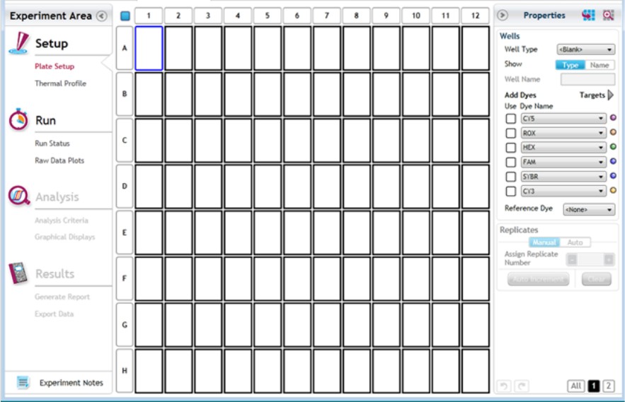
6 Setting Up the Plate
Overview of the Plate Setup screen
73 Agilent Aria Real-Time PCR Program
Overview of the Plate Setup screen
The Plate Setup screen has tools for assigning properties to the wells of
the plate so that the program can properly analyze your data.
To open the Plate Setup screen: With an experiment or project file open,
click Plate Setup in the Experiment Area panel on the left side of the
screen.

Setting Up the Plate 6
Overview of the Plate Setup screen
Agilent Aria Real-Time PCR Program 74
The plate map
In the center of the Plate Setup screen is a representation of the wells of
a 96- well plate. This diagram, called a plate map, is used for showing
which wells in the plate are in use in the current experiment, what kind
of sample is in each well, which dyes are being used for detection in the
wells, and what targets those dyes are detecting.
The properties assigned to the wells are indicated in the plate map. To see
more detailed information on the properties of a particular well, such as
target names and standard quantities, hover your cursor over the well.
You can also open a mini plate map to view the details in a selected set
of wells.
Well type
All wells that are in- use in the experiment need to be assigned a well
type. This assignment indicates to the program the type of reaction in the
well. For example, the Unknown well type is used for experimental
templates in which the quantity of the target(s) is unknown. When the
Show setting on the Plate Setup Properties panel is set to Type, the well
type appears at the top of the well.
The available well types vary depending on the experiment type.
Well name / Sample name
If desired, you can assign names to the wells of the plate. When the Show
setting on the Plate Setup Properties panel is set to Name, the well name
appears at the top of the well. The Comparative Quantitation, Allele
6 Setting Up the Plate
Overview of the Plate Setup screen
75 Agilent Aria Real-Time PCR Program
Discrimination, and User Defined experiment types also allow you to
assign sample names to designate the template sample used in each well.
The program displays the sample name at the top of each well when the
Show setting is set to Sample.
Target information
All experiment types require, at a minimum, that you designate the dyes
being used for detection in the wells. You may also assign a name to the
target being detected by each dye. If the same dye will be used to amplify
multiple targets in the experiment, assigning a unique name to each target
allows the program to distinguish between these targets during analysis.
Replicate number
If some of the wells on the plate are technical replicates of each other
(i.e., they have the exact same reaction components), you can designate
the replicate wells during plate setup by assigning them the same replicate
number. During analysis, you can choose to have the results from replicate
wells averaged together at each cycle, or you can treat replicates
separately to monitor for well- to- well variation among identical reactions.
Invalid Sets: When assigning replicates, if you see a flashing red warning
icon in the Properties panel next to Replicates, you have an invalid
replicate set on the plate. To be valid, all the wells of a set must be of the
same well type and have the same target assignments. Hover your cursor
over the warning icon to view specific information on why the program
has called a replicate set invalid.
Note that technical replicates are different from biological replicates. The
assignment of biological replicate IDs is unique to Comparative
Quantitation (and User Defined) experiments.
Reference dye
Passive reference dyes are used for normalization of the fluorescence
signal in order to compensate for non- PCR related variations in
fluorescence, such as pipetting variation from well to well. Typically, most
experiments use ROX as the reference dye.
Setting Up the Plate 6
Overview of the Plate Setup screen
Agilent Aria Real-Time PCR Program 76
If you will be adding a dye to the wells of your plate as a passive
reference dye, you need to assign a reference dye in the plate setup. The
assignment of that dye as a reference dye is indicated in the wells by the
target name REF. Note that if you assign a reference dye, you must assign
it to all wells in use on the plate.
The Properties panel
The panel on the right side of the Plate Setup screen has the tools for
assigning properties to the wells in the plate map. The content of this
panel depends on the experiment type. See the following help topics for
information on your experiment type:
“Assign plate properties for a Quantitative PCR DNA Binding Dye
experiment” on page 86
“Assign plate properties for a Quantitative PCR Fluorescence Probe
experiment” on page 94
“Assign plate properties for a Comparative Quantitation experiment” on
page 102
“Assign plate properties for an Allele Discrimination DNA Binding Dye
experiment” on page 113
“Assign plate properties for an Allele Discrimination Fluorescence Probe
experiment” on page 122
“Assign plate properties for a User Defined experiment” on page 131
To hide the Properties panel, click the arrow icon in the upper left corner
of the panel. Click the arrow again to display the Properties panel.
Additional tools for setting up a plate
Copy/Paste
To copy well information, first select the wells that contain the
information to be copied. Then, press Ctrl+c, or right- click on the plate
map and click Copy, to copy the properties of the selected wells to the
clipboard. You can later paste the properties into other wells within the
same experiment or in another open experiment.

6 Setting Up the Plate
Overview of the Plate Setup screen
77 Agilent Aria Real-Time PCR Program
To paste well information from the clipboard to a set of wells, first select
the wells that you want to paste into. Then, press Ctrl+v, or right- click on
the plate map and click Paste, to paste the well information into a
selected set of wells. You can paste into wells within the same experiment,
or into wells of an experiment that is open in another tab of the program
(provided that the properties of the wells are compatible with the
experiment type).
See “Select and view wells in the plate map” on page 79 for instructions
on selecting sub- sets of wells on the plate map.
Undo/Redo
Click the Undo icon in the lower right corner of the screen to undo your
most recent action. You can click the icon multiple times to undo multiple,
consecutive actions.
Click the Redo icon in the lower right corner of the screen to redo the
most recent action that you reversed using the Undo tool. You can click
the icon multiple times to redo multiple, consecutive actions.
You can also access the Undo and Redo commands by right- clicking
anywhere on the plate map.
Clear Selected Well or Clear Plate
To clear all the properties assigned to a well or set of wells, select the
well(s) on the plate map, right- click, and then click Clear Selected Well.
Alternatively, select the well(s) on the plate map and press Delete to clear
the properties.
To clear all properties assigned to all wells in the plate, right- click
anywhere on the plate map and click Clear Plate.

Setting Up the Plate 6
Import a plate setup
Agilent Aria Real-Time PCR Program 78
Import a plate setup
The Aria program allows you to set up the plate on the Plate Setup screen
by importing the plate setup of any existing experiment of the same
experiment type. After you import the plate setup, you can edit the well
properties as desired.
To open the Plate Setup screen: With an experiment or project file open,
click Plate Setup in the Experiment Area panel on the left side of the
screen.
To import a plate setup:
1 In the Properties panel of the Plate Setup screen, click the Import Plate
Setup icon.
The Open dialog box opens.
2 Browse to the folder of the existing experiment with the plate setup
that you want to import. Select the file and click Open.
The dialog box closes and the program imports the plate setup into the
currently open experiment.

6 Setting Up the Plate
Select and view wells in the plate map
79 Agilent Aria Real-Time PCR Program
Select and view wells in the plate map
When setting up your plate on the Plate Setup screen, you may need to
select a sub- set of wells in the 96- well plate map in order to assign
properties to specific wells. You can select and unselect wells by clicking
directly on the plate map. You may also need to view certain wells of the
plate map in more detail, which can also be done from the Plate Setup
screen.
To open the Plate Setup screen: With an experiment or project file open,
click Plate Setup in the Experiment Area panel on the left side of the
screen.
Select wells in the plate map
When a new experiment is first opened, all wells on the plate are already
selected. Selected wells appear highlighted on the plate map (see wells A1
through A6 in the image below) while unselected wells appear grayed out
(see wells A7 through A12 in the image below).
To select all wells when some wells are not already selected:
1 Click the small square in the upper left- hand corner of the plate. (If all
wells on the plate are already selected, clicking this button will unselect
all wells.)
To select an entire row or column of wells:
1 Click the corresponding row header (A–H) or column header (1–12).
To select a range of adjacent wells:
1 Click and hold the left mouse button as you drag the cursor across the
wells to be selected.
A visible marking rectangle appears.
Setting Up the Plate 6
Select and view wells in the plate map
Agilent Aria Real-Time PCR Program 80
2 When all of the required wells are included in the rectangle, release the
left mouse button.
The range of wells is selected.
To select a group of non- contiguous wells:
1 Press Ctrl as you click individually on each of the wells to be selected.
Unselect wells in the plate map
Use one of the following approaches to unselect wells:
• To unselect individual wells, press Ctrl as you click on the wells to be
unselected.
• To unselect a selected row or column, click on the header for that row
or column.
• To rapidly unselect all wells, click twice on the button in the upper
left- hand corner of the plate. This will select and then unselect all
wells.
View details of a well or wells
When the plate map is displaying all 96 wells, details such as target
names and standard quantities are not displayed. The Plate Setup screen
offers multiple ways to view the detailed properties of a single well or
multiple wells.
View details of an individual well
To view the detailed properties of an individual well:
• Hover the cursor over the well.
The program opens a larger schematic of the well that displays the
properties assigned to the well.

6 Setting Up the Plate
Select and view wells in the plate map
81 Agilent Aria Real-Time PCR Program
Zoom in/out on the plate map
You can zoom in and zoom out on the wells of the plate map using the
commands on the plate map short- cut menu.
To zoom in on the wells of the plate map:
1 Right- click anywhere on the plate map.
The short- cut menu opens.
2 Click Zoom In.
The program zooms in on the plate map, displaying fewer wells in more
detail.
3 If desired, repeat steps 1- 2 to zoom in further.
To zoom out on the wells of the plate map:
1 Right- click anywhere on the plate map.
The short- cut menu opens.
2 Click Zoom Out.
The program zooms out on the plate map.
3 If desired, repeat steps 1- 2 to zoom out until the plate map displays all
96 wells.
View a mini plate map
The minimap tool allows you to limit the plate map to specific wells,
which enables you to view more detailed information on the properties of
those wells.
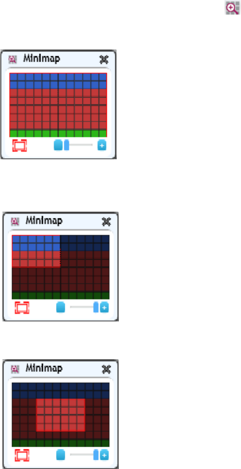
Setting Up the Plate 6
Select and view wells in the plate map
Agilent Aria Real-Time PCR Program 82
To view a mini plate map:
1 In the Properties panel, click the Minimap icon.
The Minimap box opens. This box displays a small schematic of the
plate map.
2 In the Minimap box, click the zoom scroll bar to zoom in on the wells
in the minimap.
The red box outlines the wells to be included in the minimap.
3 Click and drag the red box to capture the wells that you want to view
in more detail.

6 Setting Up the Plate
Select and view wells in the plate map
83 Agilent Aria Real-Time PCR Program
4 Click the X in the upper right corner of the Minimap box to close the
box.
The plate map on the Plate Setup screen displays only the wells
selected in the Minimap box.
To restore the mini plate map to the full 96 wells:
1 In the Properties panel, click the Minimap icon.
The Minimap box opens.

Setting Up the Plate 6
Select and view wells in the plate map
Agilent Aria Real-Time PCR Program 84
2 Click the Maximize icon in the lower left corner of the Minimap box.
3 Click the X in the upper right corner of the Minimap box to close the
box.
The plate map displays all 96 wells.
6 Setting Up the Plate
Export the plate map image
85 Agilent Aria Real-Time PCR Program
Export the plate map image
The image of the Plate Setup screen's plate map can be exported to a
Microsoft PowerPoint presentation.
To open the Plate Setup screen: With an experiment or project file open,
click Plate Setup in the Experiment Area panel on the left side of the
screen.
To export an image of the plate map to PowerPoint:
• From the Plate Setup screen, right- click anywhere on the plate map. In
the short- cut menu, click Send Image to PowerPoint.
PowerPoint opens to a new presentation file with the plate map image
on the slide.
Setting Up the Plate 6
Assign plate properties for a Quantitative PCR DNA Binding Dye experiment
Agilent Aria Real-Time PCR Program 86
Assign plate properties for a Quantitative PCR DNA Binding Dye
experiment
The controls on Plate Setup screen's Properties panel allow you to create
a customized plate setup for experiments of the type Quantitative PCR -
DNA Binding Dye Including Standard Melt.
To open the Plate Setup screen: When you create a new Quantitative
PCR experiment, you will automatically be directed to the Plate Setup
screen. To return to the Plate Setup screen at any time before, during, or
after a run, click Plate Setup in the Experiment Area panel on the left
side of the screen.
Assign well types
Use the Well Types drop- down list to assign well types to all the wells
used in the experiment. See “Well types for Quantitative PCR experiments”
on page 62 for a description of the available well types.
To assign well types:
1 On the Plate Setup screen, select all the wells in the plate map that are
of the same type. (For instructions on well selection, see “Select and
view wells in the plate map” on page 79.)
2 Select a well type from the Well Types drop- down list in the Properties
panel.
When the Show setting on the Properties panel is set to Type, the well
type appears at the top of the selected wells.
3 Repeat steps 1- 2 for all well types to be included in the experiment.
Assign well names
After you assign wells to a well type you can, if desired, assign custom
well names. Well names can be assigned manually or they can be imported
from an Excel spreadsheet or comma- delimited text file.
Assign wells to a well type before assigning well names.

6 Setting Up the Plate
Assign plate properties for a Quantitative PCR DNA Binding Dye experiment
87 Agilent Aria Real-Time PCR Program
To assign well names manually:
1 On the Properties panel of the Plate Setup screen, next to Show, select
Name.
The Well Name field becomes available for typing.
2 Select all the wells in the plate map that you want to assign to the
same well name. (For instructions on well selection, see “Select and
view wells in the plate map” on page 79.)
3 In the Well Name field, type the well name for the selected wells. Press
Enter.
The Well Name appears at the top of the selected wells.
Well names must not start with the number zero (0).
4 Repeat steps 2- 3 for all well names that you want to assign.
To assign well names by importing an Excel spreadsheet or
comma- delimited text file:
1 Create the Excel spreadsheet or comma- delimited text file and save it
to a location that is accessible while working in the Aria software.
The file must be formatted as shown below with well IDs on the left
and well names on the right. The well IDs may appear in any order but
must use the syntax A1—H12.
2 On the Plate Setup screen, right- click on the plate map. In the menu
that opens, click Import Well Name.
The Open dialog box opens.
3 At the bottom of the dialog box, use the drop- down list to select the
appropriate file type (Text, Excel Workbook, or Excel 97- 2003
Workbook).
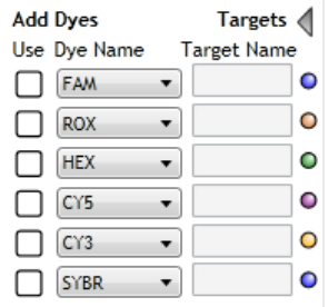
Setting Up the Plate 6
Assign plate properties for a Quantitative PCR DNA Binding Dye experiment
Agilent Aria Real-Time PCR Program 88
4 Browse to the file created in step 1. Select the file and click Open.
The software imports the well names from the file into the experiment.
A message box opens notifying you that the import was successful.
5 Click OK in the message box to close it.
The plate map displays the imported well names. For any wells that
have not yet been assigned a well type, the well name remains blanks
until a well type is assigned.
Assign dyes/targets
Use the check boxes, drop- down lists, and fields under Assign
Dyes/Targets to indicate which dyes are being used in each well and what
target each dye is detecting. Dye assignments are required, but target
name assignments are optional. If different wells will be using the same
dye to detect different targets, assigning a unique name to each target
enables the program to treat each target separately during analysis.
To assign dyes and target names:
1 On the Plate Setup screen, select all the wells in the plate map that
contain the same target. (For instructions on well selection, see “Select
and view wells in the plate map” on page 79.)
2 In the Properties panel, under Add Dyes, mark the Use check box for
the dye used for target detection in the selected wells.
3 If the fields for entering target names are not displayed, click the arrow
next to Targets.
The fields appear to the right of the dye names.

6 Setting Up the Plate
Assign plate properties for a Quantitative PCR DNA Binding Dye experiment
89 Agilent Aria Real-Time PCR Program
4 For the marked dye, type a name into the adjacent Target Name field.
The program assigns the target name to the selected wells.
If you do not assign a target name, the program uses the dye name as
the target name.
5 Repeat steps 1- 4 for all wells included in use in the experiment.
6 (Optional) Select a new color to associate with a target:
a Click the colored dot to right of the Target Name field.
b In the selection box that opens, click the desired color, or click
Advanced for more color options.
Select a reference dye
You can include a reference dye (e.g., ROX dye) to normalize the
fluorescence signal of the reporter dye.
To assign a reference dye:
• On the Plate Setup screen, select the reference dye from the Reference
Dye drop- down list in the Properties panel.
The program assigns the target name REF to all wells in use in the
experiment and displays an R ( ) in the wells of the plate map to
indicate that the well contains a reference dye.

Setting Up the Plate 6
Assign plate properties for a Quantitative PCR DNA Binding Dye experiment
Agilent Aria Real-Time PCR Program 90
Assign replicates
The Aria program uses replicate ID numbers to denote technical
replicates. Technical replicates are QPCR reaction tubes containing
identical reaction components and set up using a template from the exact
same biological sample source. While biological replicates measure the
variability in the experimental results due to uncontrolled biological
variation from sample to sample, technical replicates are used to measure
the variability in results that is introduced during the process of
experimental setup.
You can assign replicates using the Manual option or the Auto option.
When you designate replicate wells on the Plate Setup screen, you can set
the analysis criteria to average results from those wells or treat the wells
separately.
To assign replicates with the Auto option:
1 On the Plate Setup screen, select all the wells on the plate map that
have the same number of wells per replicate set.
2 In the Properties panel under Replicates, select Auto.
3 In the Direction of Assignment drop- down list, specify how the
replicate wells are arranged on the plate.
NOTE
When assigning replicates, if you see a flashing red warning icon in the Properties
panel next to Replicates, you have an invalid replicate set on the plate. To be valid,
all the wells of a set must be of the same well type and have the same target
assignments. Hover your cursor over the warning icon to view specific
information on why the program has called a replicate set invalid.

6 Setting Up the Plate
Assign plate properties for a Quantitative PCR DNA Binding Dye experiment
91 Agilent Aria Real-Time PCR Program
• Select Horizontal if the replicate reactions will be arranged
horizontally in rows.
• Select Vertical if the replicate reactions will be arranged vertically in
columns.
4 In the Wells per replicate set field, type the number of replicate wells
per reaction, or click the +/- buttons to enter the desired number.
The assigned replicate number appears in each selected well.
5 If desired, make adjustment to the auto- assignments in any of the wells
of the plate by switching to the Manual option and manually assigning
replicate numbers to those wells.
To manually assign replicates:
1 On the Plate Setup screen, select a set of wells that are part of the
same replicate set. Make sure that the selected wells are of the same
well type and contain identical targets. (For instructions on well
selection, see “Select and view wells in the plate map” on page 79.)
2 In the Properties panel under Replicates, select Manual (if not already
selected).
3 In the Assign Replicate Number field, type in the desired replicate
number for the selected wells, or click the +/- buttons to enter the
desired number.
The assigned replicate number appears in each selected well.
To assign replicates using Auto Increment:
1 On the Plate Setup screen, assign well types as needed for your
experiment.
2 In the Properties panel under Replicates, select Manual (if not already
selected).
3 Click Auto Increment.

Setting Up the Plate 6
Assign plate properties for a Quantitative PCR DNA Binding Dye experiment
Agilent Aria Real-Time PCR Program 92
When you hover your cursor anywhere on the plate map, an icon of the
number 1 appears next to the cursor.
4 With the cursor, click and drag across the group of wells that you want
to assign as replicate number 1.
The program assigns the wells to replicate number 1, and the icon next
to the cursor changes to a number 2.
5 Click and drag across the group of wells that you want to assign as
replicate number 2.
The program assigns the wells to replicate number 2, and the icon next
to the cursor changes to a number 3.
6 Continue assigning replicate numbers for the remainder of the plate.
When finished, click Auto Increment to turn off the Auto Increment
function.
Assign quantities to Standard wells
In order to generate a standard curve from your data, you need to assign
the initial template quantity to each Standard well.
To assign the standard quantities for a target in the Standard wells:
1 On the Plate Setup screen, select the Standard wells. (For instructions
on well selection, see “Select and view wells in the plate map” on
page 79.)
2 In the Properties panel under Standard Quantities, select which target
in the selected wells is the standard target (i.e., the target of known
quantity in the template).

6 Setting Up the Plate
Assign plate properties for a Quantitative PCR DNA Binding Dye experiment
93 Agilent Aria Real-Time PCR Program
3 In the Starting Amount field, type in the quantity of the standard target
present in the first replicate set of Standard wells. You will be asked to
specify the units for this amount in step 5.
4 In the drop- down list labeled A factor of, select the dilution factor
used to generate the dilution series of the standard template. For
example, if each standard quantity is separated by a factor of 10, select
10x. Negative dilution factors are used to specify a decrease in quantity
from the starting amount while positive dilution factors specify an
increase from the starting amount.
5 In the drop- down list labeled Units (for Plate), select the units of the
quantity entered in the Starting Amount field. Note that all Standard
wells on the plate must use the same units.
To clear the assigned standard quantity from one or more wells:
• Select the well(s) and click Clear.
NOTE
This quantity must be either the highest quantity or the lowest quantity in the
dilution series of the standard template sample.
Setting Up the Plate 6
Assign plate properties for a Quantitative PCR Fluorescence Probe experiment
Agilent Aria Real-Time PCR Program 94
Assign plate properties for a Quantitative PCR Fluorescence Probe
experiment
The controls on Plate Setup screen's Properties panel allow you to create
a customized plate setup for experiments of the type Quantitative PCR -
Fluorescence Probe.
To open the Plate Setup screen: When you create a new Quantitative
PCR experiment, you will automatically be directed to the Plate Setup
screen. To return to the Plate Setup screen at any time before, during, or
after a run, click Plate Setup in the Experiment Area panel on the left
side of the screen.
Assign well types
Use the Well Types drop- down list to assign well types to all the wells
used in the experiment. See “Well types for Quantitative PCR experiments”
on page 62 for a description of the available well types.
To assign well types:
1 On the Plate Setup screen, select all the wells in the plate map that are
of the same type. (For instructions on well selection, see “Select and
view wells in the plate map” on page 79.)
2 Select a well type from the Well Types drop- down list in the Properties
panel.
When the Show setting on the Properties panel is set to Type, the well
type appears at the top of the selected wells.
3 Repeat steps 1 and 2 for all well types to be included in the
experiment.
Assign well names
After you assign wells to a well type you can, if desired, assign custom
well names. Well names can be assigned manually or they can be imported
from an Excel spreadsheet or comma- delimited text file.
Assign wells to a well type before assigning well names.

6 Setting Up the Plate
Assign plate properties for a Quantitative PCR Fluorescence Probe experiment
95 Agilent Aria Real-Time PCR Program
To assign well names manually:
1 On the Properties panel of the Plate Setup screen, next to Show, select
Name.
The Well Name field becomes available for typing.
2 Select all the wells in the plate map that you want to assign to the
same well name. (For instructions on well selection, see “Select and
view wells in the plate map” on page 79.)
You must assign a well to a well type before you can assign it a well
name.
3 In the Well Name field, type the well name for the selected wells. Press
Enter.
The Well Name appears at the top of the selected wells.
Well names must not start with the number zero (0).
4 Repeat steps 2- 3 for all well names that you want to assign.
To assign well names by importing an Excel spreadsheet or
comma- delimited text file:
1 Create the Excel spreadsheet or comma- delimited text file and save it
to a location that is accessible while working in the Aria software.
The file must be formatted as shown below with well IDs on the left
and well names on the right. The well IDs may appear in any order but
must use the syntax A1—H12.
2 On the Plate Setup screen, right- click on the plate map. In the menu
that opens, click Import Well Name.
The Open dialog box opens.

Setting Up the Plate 6
Assign plate properties for a Quantitative PCR Fluorescence Probe experiment
Agilent Aria Real-Time PCR Program 96
3 At the bottom of the dialog box, use the drop- down list to select the
appropriate file type (Text, Excel Workbook, or Excel 97- 2003
Workbook).
4 Browse to the file created in step 1. Select the file and click Open.
The software imports the well names from the file into the experiment.
A message box opens notifying you that the import was successful.
5 Click OK in the message box to close it.
The plate map displays the imported well names. For any wells that
have not yet been assigned a well type, the well name remains blanks
until a well type is assigned.
Assign dyes/targets
Use the check boxes, drop- down lists, and fields under Assign
Dyes/Targets to indicate which dyes are being used in each well and what
target each dye is detecting. Dye assignments are required, but target
name assignments are optional. If different wells will be using the same
dye to detect different targets, assigning a unique name to each target
enables the program to treat each target separately during analysis.
To assign dyes and target names:
1 On the Plate Setup screen, select all the wells in the plate map that
contain the same target. (For instructions on well selection, see “Select
and view wells in the plate map” on page 79.)
2 Under Add Dyes, mark the Use check boxes for the dyes used for target
detection in the selected wells.

6 Setting Up the Plate
Assign plate properties for a Quantitative PCR Fluorescence Probe experiment
97 Agilent Aria Real-Time PCR Program
3 If the fields for entering target names are not displayed, click the arrow
next to Targets.
The fields appear to the right of the dye names.
4 For the marked dyes, type a name into the adjacent Target Name field.
The program assigns the target names to the selected wells.
If you do not assign a target name to a marked dye, the program uses
the dye name as the target name.
5 Repeat steps 1- 4 for all wells included in use in the experiment.
6 (Optional) Select a new color to associate with a target:
a Click the colored dot to right of the Target Name field.
b In the selection box that opens, click the desired color, or click
Advanced for more color options.
Select a reference dye
You can include a reference dye (e.g., ROX dye) to normalize the
fluorescence signal of the reporter dye.
To assign a reference dye:
• On the Plate Setup screen, select the reference dye from the Reference
Dye drop- down list in the Properties panel.
The program assigns the target name REF to all wells in use in the
experiment and displays an R ( ) in the wells of the plate map to
indicate that the well contains a reference dye.

Setting Up the Plate 6
Assign plate properties for a Quantitative PCR Fluorescence Probe experiment
Agilent Aria Real-Time PCR Program 98
Assign replicates
Replicates are wells that contain identical reaction components (repeats).
You can assign replicates using the Manual option or the Auto option.
When you designate replicate wells on the Plate Setup screen, you can set
the analysis criteria to average results from those wells or treat the wells
separately.
To assign replicates with the Auto option:
1 On the Plate Setup screen, select all the wells on the plate map that
have the same number of wells per replicate set.
2 In the Properties panel under Replicates, select Auto.
3 In the Direction of Assignment drop- down list, specify how the
replicate wells are arranged on the plate.
• Select Horizontal if the replicate reactions will be arranged
horizontally in rows.
• Select Vertical if the replicate reactions will be arranged vertically in
columns.
4 In the Wells per replicate set field, type the number of replicate wells
per reaction, or click the +/- buttons to enter the desired number.
The assigned replicate number appears in each selected well.
NOTE
When assigning replicates, if you see a flashing red warning icon in the Properties
panel next to Replicates, you have an invalid replicate set on the plate. To be valid,
all the wells of a set must be of the same well type and have the same target
assignments. Hover your cursor over the warning icon to view specific
information on why the program has called a replicate set invalid.

6 Setting Up the Plate
Assign plate properties for a Quantitative PCR Fluorescence Probe experiment
99 Agilent Aria Real-Time PCR Program
5 If desired, make adjustment to the auto- assignments in any of the wells
of the plate by switching to the Manual option and manually assigning
replicate numbers to those wells.
To manually assign replicates:
1 On the Plate Setup screen, select a set of wells that are part of the
same replicate set. Make sure that the selected wells are of the same
well type and contain identical targets. (For instructions on well
selection, see “Select and view wells in the plate map” on page 79.)
2 In the Properties panel under Replicates, select Manual (if not already
selected).
3 In the Assign Replicate Number field, type in the desired replicate
number for the selected wells, or click the +/- buttons to enter the
desired number.
The assigned replicate number appears in each selected well.
To assign replicates using Auto Increment:
1 On the Plate Setup screen, assign well types as needed for your
experiment.
2 In the Properties panel under Replicates, select Manual (if not already
selected).
3 Click Auto Increment.
When you hover your cursor anywhere on the plate map, an icon of the
number 1 appears next to the cursor.
4 With the cursor, click and drag across the group of wells that you want
to assign as replicate number 1.

Setting Up the Plate 6
Assign plate properties for a Quantitative PCR Fluorescence Probe experiment
Agilent Aria Real-Time PCR Program 100
The program assigns the wells to replicate number 1, and the icon next
to the cursor changes to a number 2.
5 Click and drag across the group of wells that you want to assign as
replicate number 2.
The program assigns the wells to replicate number 2, and the icon next
to the cursor changes to a number 3.
6 Continue assigning replicate numbers for the remainder of the plate.
When finished, click Auto Increment to turn off the Auto Increment
function.
Assign quantities to Standard wells
In order to generate a standard curve from your data, you need to assign
the initial template quantity to each Standard well.
To assign the standard quantities for a target in the Standard wells:
1 On the Plate Setup screen, select the Standard wells. (For instructions
on well selection, see “Select and view wells in the plate map” on
page 79.)
2 In the Properties panel under Standard Quantities, select which target
in the selected wells is the standard target (i.e., the target of known
quantity in the template).
3 In the Starting Amount field, type in the quantity of the standard target
present in the first replicate set of Standard wells. You will be asked to
specify the units for this amount in step 5.
NOTE
This quantity must be either the highest quantity or the lowest quantity in the
dilution series of the standard template sample.
6 Setting Up the Plate
Assign plate properties for a Quantitative PCR Fluorescence Probe experiment
101 Agilent Aria Real-Time PCR Program
4 In the drop- down list labeled A factor of, select the dilution factor
used to generate the dilution series of the standard template. For
example, if each standard quantity is separated by a factor of 10, select
10x. Negative dilution factors are used to specify a decrease in quantity
from the starting amount while positive dilution factors specify an
increase from the starting amount.
5 In the drop- down list labeled Units (for Plate), select the units of the
quantity entered in the Starting Amount field. Note that all Standard
wells on the plate must use the same units.
To clear the assigned standard quantity from one or more wells:
• Select the well(s) and click Clear.

Setting Up the Plate 6
Assign plate properties for a Comparative Quantitation experiment
Agilent Aria Real-Time PCR Program 102
Assign plate properties for a Comparative Quantitation experiment
The program analyzes comparative quantitation data based on how the
targets and well types are assigned in the Plate Setup screen. For a
particular target- of- interest, the program measures the quantity of the
target in an Unknown well relative to the level of that target in the
Calibrator well.
To open the Plate Setup screen: When you create a new Comparative
Quantitation experiment, you will automatically be directed to the Plate
Setup screen. To return to the Plate Setup screen at any time before,
during, or after a run, click Plate Setup in the Experiment Area panel on
the left side of the screen.
Assign well types
Use the Well Types drop- down list to assign well types to all the wells
used in the experiment. See “Well types for Comparative Quantitation
experiments” on page 66 for a description of the available well types.
To assign well types:
1 On the Plate Setup screen, select all the wells in the plate map that are
of the same type. (For instructions on well selection, see “Select and
view wells in the plate map” on page 79.)
2 Select a well type from the Well Types drop- down list in the Properties
panel.
When the Show setting on the Properties panel is set to Type, the well
type appears at the top of the selected wells.
3 Repeat steps 1 and 2 for all well types to be included in the
experiment.
NOTE
In comparative quantitation, it is important for the amplification efficiencies of the
target-of-interest and the normalizer target to be reproducible and, ideally, very
similar. If you do not know the amplification efficiency for all of your targets, run a
standard curve. See“Determining amplification efficiencies for the targets of
interest and normalizer targets” on page 64 for more information.

6 Setting Up the Plate
Assign plate properties for a Comparative Quantitation experiment
103 Agilent Aria Real-Time PCR Program
Assign well names
After you assign wells to a well type you can, if desired, assign custom
well names. Well names can be assigned manually or they can be imported
from an Excel spreadsheet or comma- delimited text file.
Assign wells to a well type before assigning well names.
To assign well names manually:
1 On the Properties panel of the Plate Setup screen, next to Show, select
Name.
The Well Name field becomes available for typing.
2 Select all the wells in the plate map that you want to assign to the
same well name. (For instructions on well selection, see “Select and
view wells in the plate map” on page 79.)
You must assign a well to a well type before you can assign it a well
name.
3 In the Well Name field, type the well name for the selected wells. Press
Enter.
The Well Name appears at the top of the selected wells.
Well names must not start with the number zero (0).
4 Repeat steps 2- 3 for all well names that you want to assign.
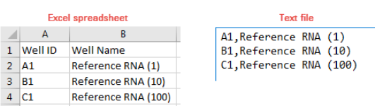
Setting Up the Plate 6
Assign plate properties for a Comparative Quantitation experiment
Agilent Aria Real-Time PCR Program 104
To assign well names by importing an Excel spreadsheet or
comma- delimited text file:
1 Create the Excel spreadsheet or comma- delimited text file and save it
to a location that is accessible while working in the Aria software.
The file must be formatted as shown below with well IDs on the left
and well names on the right. The well IDs may appear in any order but
must use the syntax A1—H12.
2 On the Plate Setup screen, right- click on the plate map. In the menu
that opens, click Import Well Name.
The Open dialog box opens.
3 At the bottom of the dialog box, use the drop- down list to select the
appropriate file type (Text, Excel Workbook, or Excel 97- 2003
Workbook).
4 Browse to the file created in step 1. Select the file and click Open.
The software imports the well names from the file into the experiment.
A message box opens notifying you that the import was successful.
5 Click OK in the message box to close it.
The plate map displays the imported well names. For any wells that
have not yet been assigned a well type, the well name remains blanks
until a well type is assigned.
Assign sample names and biological replicates
Once well types have been assigned, you can specify the sample in each
well by assigning sample names. Each unique template sample included in
the experiment can be assigned its own sample name. If the normalizer
target and the target- of- interest are being amplified in different wells,
be sure to assign the same sample name to these wells so the data are
normalized properly during analysis.

6 Setting Up the Plate
Assign plate properties for a Comparative Quantitation experiment
105 Agilent Aria Real-Time PCR Program
For samples that are biological replicates, assign the same sample name to
the wells but give the wells different biological replicate ID numbers to
keep them differentiated. Biological replicates are template samples that
were isolated independently but from biologically- identical sources (see
“Including biological replicates in comparative quantitation” on page 65 for
more information on biological replicates).
To assign sample names manually:
1 On the Properties panel of the Plate Setup screen, next to Show, select
Sample.
The Sample Name field becomes available for typing.
2 Select a group of wells that contain the same template sample or a
group of wells containing samples that are biological replicates. (For
instructions on well selection, see “Select and view wells in the plate
map” on page 79.)
3 In the Sample Name field, type in a name for the sample. Press Enter.
The sample name appears at the top the selected wells.
Sample names must not start with the number zero (0).
4 Repeat steps 2- 3 for all samples to be included in the experiment.
To assign sample names in batch mode (using barcode reader or manual
input):
1 If inputting sample names with a barcode reader, set up the barcode
reader and barcodes.
The barcodes correspond to the sample names to be inputted into the
plate setup. Each time you read a barcode, it is inputted into the Aria
software as the sample name for the selected well.
a Connect the barcode reader directly to the PC on which the Aria
software is installed.
b Make sure the barcodes are within reach of the barcode scanner.
Setting Up the Plate 6
Assign plate properties for a Comparative Quantitation experiment
Agilent Aria Real-Time PCR Program 106
2 On the Plate Setup screen, assign wells to a well type before assigning
sample names in batch mode.
3 Select all the wells to which you want to assign sample names. (For
instructions on well selection, see “Select and view wells in the plate
map” on page 79.)
4 Right- click on the plate map. In the menu that opens, click Input
Sample Name in Batch Mode.
Next to Show, the Sample option is automatically selected and the
cursor is in the Sample Name field.
The first well among the group of selected wells is actively selected for
input, as indicating by the flashing outline around the well.
5 Input the sample name for the actively selected well.
• If inputting sample names using a barcode reader, scan the barcode
corresponding to the sample name.
• If inputting sample names manually, type the sample name then
press Enter.
The inputted sample name is assigned. The next well among the group
of selected wells is now actively selected for input.
6 Repeat step 5 for all selected wells to be assigned a sample name.
7 After inputting the sample name for the last selected well, right- click on
the plate map. In the menu that opens, clear the check box next to
Input Sample Name in Batch Mode.
To assign biological replicate ID numbers:
1 On the Properties panel of the Plate Setup screen, next to Show, select
Sample.
The Biological Replicate ID field becomes available for typing.
2 Among a group of biological replicate wells, select the first sub- set of
wells that require the same biological replicate ID. (A separate ID is to
be assigned to each biological replicate sample within the group.)
3 In the Biological Replicate ID field, type in a number to be assigned to
the selected wells. Press Enter.
The program adds the biological replicate ID number to the end of the
sample name at the top of the selected well(s).
4 Repeat steps 2- 3 for the remaining wells that require a biological
replicate ID assignment.
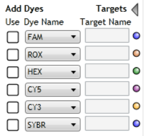
6 Setting Up the Plate
Assign plate properties for a Comparative Quantitation experiment
107 Agilent Aria Real-Time PCR Program
Assign dyes/targets
Use the check boxes, drop- down lists, and fields under Assign
Dyes/Targets to indicate which dyes are being used in each well and what
target each dye is detecting. Dye assignments are required, but target
name assignments are optional. If different wells will be using the same
dye to detect different targets, assigning a unique name to each target
enables the program to treat each target separately during analysis.
To assign dyes and target names:
1 On the Plate Setup screen, select all the wells in the plate map that
contain the same target. (For instructions on well selection, see “Select
and view wells in the plate map” on page 79.)
2 Under Add Dyes, mark the Use check boxes for the dyes used for target
detection in the selected wells.
3 If the fields for entering target names are not displayed, click the arrow
next to Targets.
The fields appear to the right of the dye names.
4 For the marked dyes, type a name into the adjacent Target Name field.
The program assigns the target names to the selected wells.
If you do not assign a target name to a marked dye, the program uses
the dye name as the target name.
5 Repeat steps 1- 4 for all wells included in use in the experiment.
6 (Optional) Select a new color to associate with a target:
a Click the colored dot to right of the Target Name field.
b In the selection box that opens, click the desired color, or click
Advanced for more color options.

Setting Up the Plate 6
Assign plate properties for a Comparative Quantitation experiment
Agilent Aria Real-Time PCR Program 108
Select a reference dye
You can include a reference dye (e.g., ROX dye) to normalize the
fluorescence signal of the reporter dye.
To assign a reference dye:
• On the Plate Setup screen, select the reference dye from the Reference
Dye drop- down list in the Properties panel.
The program assigns the target name REF to all wells in use in the
experiment and displays an R ( ) in the wells of the plate map to
indicate that the well contains a reference dye.
Designate the normalizer
In order to normalize the quantity level of your target- of- interest to a
normalizer target, you need to amplify the normalizer in both the
Unknown wells and the Calibrator wells. You can amplify the normalizer
in the same well as the target- of- interest (if the two targets are detected
with spectrally distinct dyes) or you can amplify them in separate wells
that contain the same template sample.
When you designate multiple normalizers in the same well, the program
first calculates the normalized target- of- interest levels for each normalizer
separately, and then calculates the geometric mean of all normalized
values. The program then uses the geometric mean for the Relative
Quantity calculations.
To assign a normalizer target:
1 On the Plate Setup screen, select the wells that will be used for
amplification of the normalizer target.
2 In the Normalizer Dye drop- down list on the Properties panel, select
the dye (or dyes) that is to be used for detection of the normalizer
target.
The program assigns the target name NORM to the selected wells and
displays an N in the wells on the plate map.

6 Setting Up the Plate
Assign plate properties for a Comparative Quantitation experiment
109 Agilent Aria Real-Time PCR Program
Assign replicates
Replicates are wells that contain identical reaction components (repeats).
You can assign replicates using the Manual option or the Auto option.
When you designate replicate wells on the Plate Setup screen, you can set
the analysis criteria to average results from those wells or treat the wells
separately.
To assign replicates with the Auto option:
1 On the Plate Setup screen, select all the wells on the plate map that
have the same number of wells per replicate set.
2 In the Properties panel under Replicates, select Auto.
3 In the Direction of Assignment drop- down list, specify how the
replicate wells are arranged on the plate.
• Select Horizontal if the replicate reactions will be arranged
horizontally in rows.
• Select Vertical if the replicate reactions will be arranged vertically in
columns.
4 In the Wells per replicate set field, type the number of replicate wells
per reaction, or click the +/- buttons to enter the desired number.
NOTE
When assigning replicates, if you see a flashing red warning icon in the Properties
panel next to Replicates, you have an invalid replicate set on the plate. To be valid,
all the wells of a set must be of the same well type and have the same target
assignments. Hover your cursor over the warning icon to view specific
information on why the program has called a replicate set invalid.

Setting Up the Plate 6
Assign plate properties for a Comparative Quantitation experiment
Agilent Aria Real-Time PCR Program 110
The assigned replicate number appears in each selected well.
5 If desired, make adjustment to the auto- assignments in any of the wells
of the plate by switching to the Manual option and manually assigning
replicate numbers to those wells.
To manually assign replicates:
1 On the Plate Setup screen, select a set of wells that are part of the
same replicate set. Make sure that the selected wells are of the same
well type and contain identical targets. (For instructions on well
selection, see “Select and view wells in the plate map” on page 79.)
2 In the Properties panel under Replicates, select Manual (if not already
selected).
3 In the Assign Replicate Number field, type in the desired replicate
number for the selected wells, or click the +/- buttons to enter the
desired number.
The assigned replicate number appears in each selected well.
To assign replicates using Auto Increment:
1 On the Plate Setup screen, assign well types as needed for your
experiment.
2 In the Properties panel under Replicates, select Manual (if not already
selected).
3 Click Auto Increment.
When you hover your cursor anywhere on the plate map, an icon of the
number 1 appears next to the cursor.
4 With the cursor, click and drag across the group of wells that you want
to assign as replicate number 1.

6 Setting Up the Plate
Assign plate properties for a Comparative Quantitation experiment
111 Agilent Aria Real-Time PCR Program
The program assigns the wells to replicate number 1, and the icon next
to the cursor changes to a number 2.
5 Click and drag across the group of wells that you want to assign as
replicate number 2.
The program assigns the wells to replicate number 2, and the icon next
to the cursor changes to a number 3.
6 Continue assigning replicate numbers for the remainder of the plate.
When finished, click Auto Increment to turn off the Auto Increment
function.
Assign quantities to Standard wells
If your Comparative Quantitation experiment includes running a set of
standards in order to calculate amplification efficiencies of your targets,
you need to assign the initial template quantity to each Standard well.
To assign the standard quantities for a target in the Standard wells:
1 On the Plate Setup screen, select the Standard wells. (For instructions
on well selection, see “Select and view wells in the plate map” on
page 79.)
2 In the Properties panel under Standard Quantities, select which target
in the selected wells is the standard target (i.e., the target of known
quantity in the template).
3 In the Starting Amount field, type in the quantity of the standard target
present in the first replicate set of Standard wells. You will be asked to
specify the units for this amount in step 5.
NOTE
This quantity must be either the highest quantity or the lowest quantity in the
dilution series of the standard template sample.
Setting Up the Plate 6
Assign plate properties for a Comparative Quantitation experiment
Agilent Aria Real-Time PCR Program 112
4 In the drop- down list labeled A factor of, select the dilution factor
used to generate the dilution series of the standard template. For
example, if each standard quantity is separated by a factor of 10, select
10x. Negative dilution factors are used to specify a decrease in quantity
from the starting amount while positive dilution factors specify an
increase from the starting amount.
5 In the drop- down list labeled Units (for Plate), select the units of the
quantity entered in the Starting Amount field. Note that all Standard
wells on the plate must use the same units.
To clear the assigned standard quantity from one or more wells:
• Select the well(s) and click Clear.
6 Setting Up the Plate
Assign plate properties for an Allele Discrimination DNA Binding Dye experiment
113 Agilent Aria Real-Time PCR Program
Assign plate properties for an Allele Discrimination DNA Binding Dye
experiment
The controls on Plate Setup screen's Properties panel allow you to create
a customized plate setup for experiments of the type Allele
Discrimination - DNA Binding Dye Including High Resolution Melt.
To open the Plate Setup screen: When you create a new Allele
Discrimination experiment, you will automatically be directed to the Plate
Setup screen. To return to the Plate Setup screen at any time before,
during, or after a run, click Plate Setup in the Experiment Area panel on
the left side of the screen.
Assign well types
Use the Well Types drop- down list to assign well types to all the wells
used in the experiment. See “Well types for Allele Discrimination - DNA
Binding Dye experiments” on page 68 for a description of the available
well types.
To assign well types:
1 On the Plate Setup screen, select all the wells in the plate map that are
of the same type. (For instructions on well selection, see “Select and
view wells in the plate map” on page 79.)
2 Select a well type from the Well Types drop- down list in the Properties
panel.
When the Show setting on the Properties panel is set to Type, the well
type appears at the top of the selected wells.
3 Repeat steps 1 and 2 for all well types to be included in the
experiment.
Assign well names
After you assign wells to a well type you can, if desired, assign custom
well names. Well names can be assigned manually or they can be imported
from an Excel spreadsheet or comma- delimited text file.
Assign wells to a well type before assigning well names.

Setting Up the Plate 6
Assign plate properties for an Allele Discrimination DNA Binding Dye experiment
Agilent Aria Real-Time PCR Program 114
To assign well names manually:
1 On the Properties panel of the Plate Setup screen, next to Show, select
Name.
The Well Name field becomes available for typing.
2 Select all the wells in the plate map that you want to assign to the
same well name. (For instructions on well selection, see “Select and
view wells in the plate map” on page 79.)
You must assign a well to a well type before you can assign it a well
name.
3 In the Well Name field, type the well name for the selected wells. Press
Enter.
The Well Name appears at the top of the selected wells.
Well names must not start with the number zero (0).
4 Repeat steps 2- 3 for all well names that you want to assign.
To assign well names by importing an Excel spreadsheet or
comma- delimited text file:
1 Create the Excel spreadsheet or comma- delimited text file and save it
to a location that is accessible while working in the Aria software.
The file must be formatted as shown below with well IDs on the left
and well names on the right. The well IDs may appear in any order but
must use the syntax A1—H12.
2 On the Plate Setup screen, right- click on the plate map. In the menu
that opens, click Import Well Name.
The Open dialog box opens.

6 Setting Up the Plate
Assign plate properties for an Allele Discrimination DNA Binding Dye experiment
115 Agilent Aria Real-Time PCR Program
3 At the bottom of the dialog box, use the drop- down list to select the
appropriate file type (Text, Excel Workbook, or Excel 97- 2003
Workbook).
4 Browse to the file created in step 1. Select the file and click Open.
The software imports the well names from the file into the experiment.
A message box opens notifying you that the import was successful.
5 Click OK in the message box to close it.
The plate map displays the imported well names. For any wells that
have not yet been assigned a well type, the well name remains blanks
until a well type is assigned.
Assign sample names
After you assign well types, you can specify the sample in each well by
assigning sample names. Each unique template sample included in the
experiment can be assigned its own sample name.
To assign sample names manually:
1 On the Properties panel of the Plate Setup screen, next to Show, select
Sample.
The Sample Name field becomes available for typing.
2 Select all the wells in the plate map that contain the same template
sample. (For instructions on well selection, see “Select and view wells
in the plate map” on page 79.)
3 In the Sample Name field, type in a name for the sample. Press Enter.
The sample name appears at the top of the selected wells.
Sample names must not start with the number zero (0).
4 Repeat steps 2- 3 for all samples to be included in the experiment.
Setting Up the Plate 6
Assign plate properties for an Allele Discrimination DNA Binding Dye experiment
Agilent Aria Real-Time PCR Program 116
To assign sample names in batch mode (using barcode reader or manual
input):
1 If inputting sample names with a barcode reader, set up the barcode
reader and barcodes.
The barcodes correspond to the sample names to be inputted into the
plate setup. Each time you read a barcode, it is inputted into the Aria
software as the sample name for the selected well.
a Connect the barcode reader directly to the PC on which the Aria
software is installed.
b Make sure the barcodes are within reach of the barcode scanner.
2 On the Plate Setup screen, assign wells to a well type before assigning
sample names in batch mode.
3 Select all the wells to which you want to assign sample names. (For
instructions on well selection, see “Select and view wells in the plate
map” on page 79.)
4 Right- click on the plate map. In the menu that opens, click Input
Sample Name in Batch Mode.
Next to Show, the Sample option is automatically selected and the
cursor is in the Sample Name field.
The first well among the group of selected wells is actively selected for
input, as indicating by the flashing outline around the well.
5 Input the sample name for the actively selected well.
• If inputting sample names using a barcode reader, scan the barcode
corresponding to the sample name.
• If inputting sample names manually, type the sample name then
press Enter.
The inputted sample name is assigned. The next well among the group
of selected wells is now actively selected for input.
6 Repeat step 5 for all selected wells to be assigned a sample name.
7 After inputting the sample name for the last selected well, right- click on
the plate map. In the menu that opens, clear the check box next to
Input Sample Name in Batch Mode.

6 Setting Up the Plate
Assign plate properties for an Allele Discrimination DNA Binding Dye experiment
117 Agilent Aria Real-Time PCR Program
Assign dyes/targets
Use the check boxes, drop- down lists, and fields under Assign
Dyes/Targets to indicate which dyes are being used in each well and what
target each dye is detecting. Dye assignments are required, but target
name assignments are optional. If different wells will be using the same
dye to detect different targets, assigning a unique name to each target
enables the program to treat each target separately during analysis.
To assign dyes and target names:
1 On the Plate Setup screen, select all the wells in the plate map that
contain the same target. (For instructions on well selection, see “Select
and view wells in the plate map” on page 79.)
2 Under Add Dyes, mark the Use check box for the dye used for target
detection in the selected wells.
3 If the fields for entering target names are not displayed, click the arrow
next to Targets.
The fields appear to the right of the dye names.
4 For the marked dye, type a name into the adjacent Target Name field.
The program assigns the target name to the selected wells.
If you do not assign a target name, the program uses the dye name as
the target name.
5 Repeat steps 1- 4 for all wells included in use in the experiment.

Setting Up the Plate 6
Assign plate properties for an Allele Discrimination DNA Binding Dye experiment
Agilent Aria Real-Time PCR Program 118
6 (Optional) Select a new color to associate with a target:
a Click the colored dot to right of the Target Name field.
b In the selection box that opens, click the desired color, or click
Advanced for more color options.
Select a reference dye
You can include a reference dye (e.g., ROX dye) to normalize the
fluorescence signal of the reporter dye.
To assign a reference dye:
• On the Plate Setup screen, select the reference dye from the Reference
Dye drop- down list in the Properties panel.
The program assigns the target name REF to all wells in use in the
experiment and displays an R ( ) in the wells of the plate map to
indicate that the well contains a reference dye.

6 Setting Up the Plate
Assign plate properties for an Allele Discrimination DNA Binding Dye experiment
119 Agilent Aria Real-Time PCR Program
Assign replicates
Replicates are wells that contain identical reaction components (repeats).
You can assign replicates using the Manual option or the Auto option.
When you designate replicate wells on the Plate Setup screen, you can set
the analysis criteria to average results from those wells or treat the wells
separately.
To assign replicates with the Auto option:
1 On the Plate Setup screen, select all the wells on the plate map that
have the same number of wells per replicate set.
2 In the Properties panel under Replicates, select Auto.
3 In the Direction of Assignment drop- down list, specify how the
replicate wells are arranged on the plate.
• Select Horizontal if the replicate reactions will be arranged
horizontally in rows.
• Select Vertical if the replicate reactions will be arranged vertically in
columns.
4 In the Wells per replicate set field, type the number of replicate wells
per reaction, or click the +/- buttons to enter the desired number.
The assigned replicate number appears in each selected well.
NOTE
When assigning replicates, if you see a flashing red warning icon in the Properties
panel next to Replicates, you have an invalid replicate set on the plate. To be valid,
all the wells of a set must be of the same well type and have the same target
assignments. Hover your cursor over the warning icon to view specific
information on why the program has called a replicate set invalid.

Setting Up the Plate 6
Assign plate properties for an Allele Discrimination DNA Binding Dye experiment
Agilent Aria Real-Time PCR Program 120
5 If desired, make adjustment to the auto- assignments in any of the wells
of the plate by switching to the Manual option and manually assigning
replicate numbers to those wells.
To manually assign replicates:
1 On the Plate Setup screen, select a set of wells that are part of the
same replicate set. Make sure that the selected wells are of the same
well type and contain identical targets. (For instructions on well
selection, see “Select and view wells in the plate map” on page 79.)
2 In the Properties panel under Replicates, select Manual (if not already
selected).
3 In the Assign Replicate Number field, type in the desired replicate
number for the selected wells, or click the +/- buttons to enter the
desired number.
The assigned replicate number appears in each selected well.
To assign replicates using Auto Increment:
1 On the Plate Setup screen, assign well types as needed for your
experiment.
2 In the Properties panel under Replicates, select Manual (if not already
selected).
3 Click Auto Increment.
When you hover your cursor anywhere on the plate map, an icon of the
number 1 appears next to the cursor.
4 With the cursor, click and drag across the group of wells that you want
to assign as replicate number 1.
6 Setting Up the Plate
Assign plate properties for an Allele Discrimination DNA Binding Dye experiment
121 Agilent Aria Real-Time PCR Program
The program assigns the wells to replicate number 1, and the icon next
to the cursor changes to a number 2.
5 Click and drag across the group of wells that you want to assign as
replicate number 2.
The program assigns the wells to replicate number 2, and the icon next
to the cursor changes to a number 3.
6 Continue assigning replicate numbers for the remainder of the plate.
When finished, click Auto Increment to turn off the Auto Increment
function.
Setting Up the Plate 6
Assign plate properties for an Allele Discrimination Fluorescence Probe experiment
Agilent Aria Real-Time PCR Program 122
Assign plate properties for an Allele Discrimination Fluorescence Probe
experiment
The controls on Plate Setup screen's Properties panel allow you to create
a customized plate setup for experiments of the type Allele
Discrimination - Fluorescence Probe.
To open the Plate Setup screen: When you create a new Allele
Discrimination experiment, you will automatically be directed to the Plate
Setup screen. To return to the Plate Setup screen at any time before,
during, or after a run, click Plate Setup in the Experiment Area panel on
the left side of the screen.
Assign well types
Use the Well Types drop- down list to assign well types to all the wells
used in the experiment. See “Well types for Allele Discrimination -
Fluorescence Probe experiments” on page 70 for a description of the
available well types.
To assign well types:
1 On the Plate Setup screen, select all the wells in the plate map that are
of the same type. (For instructions on well selection, see “Select and
view wells in the plate map” on page 79.)
2 Select a well type from the Well Types drop- down list in the Properties
panel.
When the Show setting on the Properties panel is set to Type, the well
type appears at the top of the selected wells.
3 Repeat steps 1 through 2 for all well types to be included in the
experiment.
Assign well names
After you assign wells to a well type you can, if desired, assign custom
well names. Well names can be assigned manually or they can be imported
from an Excel spreadsheet or comma- delimited text file.
Assign wells to a well type before assigning well names.

6 Setting Up the Plate
Assign plate properties for an Allele Discrimination Fluorescence Probe experiment
123 Agilent Aria Real-Time PCR Program
To assign well names manually:
1 On the Properties panel of the Plate Setup screen, next to Show, select
Name.
The Well Name field becomes available for typing.
2 Select all the wells in the plate map that you want to assign to the
same well name. (For instructions on well selection, see “Select and
view wells in the plate map” on page 79.)
You must assign a well to a well type before you can assign it a well
name.
3 In the Well Name field, type the well name for the selected wells. Press
Enter.
The Well Name appears at the top of the selected wells.
Well names must not start with the number zero (0).
4 Repeat steps 2- 3 for all well names that you want to assign.
To assign well names by importing an Excel spreadsheet or
comma- delimited text file:
1 Create the Excel spreadsheet or comma- delimited text file and save it
to a location that is accessible while working in the Aria software.
The file must be formatted as shown below with well IDs on the left
and well names on the right. The well IDs may appear in any order but
must use the syntax A1—H12.
2 On the Plate Setup screen, right- click on the plate map. In the menu
that opens, click Import Well Name.
The Open dialog box opens.

Setting Up the Plate 6
Assign plate properties for an Allele Discrimination Fluorescence Probe experiment
Agilent Aria Real-Time PCR Program 124
3 At the bottom of the dialog box, use the drop- down list to select the
appropriate file type (Text, Excel Workbook, or Excel 97- 2003
Workbook).
4 Browse to the file created in step 1. Select the file and click Open.
The software imports the well names from the file into the experiment.
A message box opens notifying you that the import was successful.
5 Click OK in the message box to close it.
The plate map displays the imported well names. For any wells that
have not yet been assigned a well type, the well name remains blanks
until a well type is assigned.
Assign sample names
After you assign well types, you can specify the sample in each well by
assigning sample names. Each unique template sample included in the
experiment can be assigned its own sample name. If the two alleles are
being amplified in separate wells, the sample name is used to associate
the wells amplifying Allele A with the wells amplifying Allele B from the
same template.
To assign sample names manually:
1 On the Properties panel of the Plate Setup screen, next to Show, select
Sample.
The Sample Name field becomes available for typing.
2 Select all the wells in the plate map that contain the same template
sample. (For instructions on well selection, see “Select and view wells
in the plate map” on page 79.)
3 In the Sample Name field, type in a name for the sample. Press Enter.
The sample name appears at the top of the selected wells.
Sample names must not start with the number zero (0).
4 Repeat steps 2- 3 for all samples to be included in the experiment.
6 Setting Up the Plate
Assign plate properties for an Allele Discrimination Fluorescence Probe experiment
125 Agilent Aria Real-Time PCR Program
To assign sample names in batch mode (using barcode reader or manual
input):
1 If inputting sample names with a barcode reader, set up the barcode
reader and barcodes.
The barcodes correspond to the sample names to be inputted into the
plate setup. Each time you read a barcode, it is inputted into the Aria
software as the sample name for the selected well.
a Connect the barcode reader directly to the PC on which the Aria
software is installed.
b Make sure the barcodes are within reach of the barcode scanner.
2 On the Plate Setup screen, assign wells to a well type before assigning
sample names in batch mode.
3 Select all the wells to which you want to assign sample names. (For
instructions on well selection, see “Select and view wells in the plate
map” on page 79.)
4 Right- click on the plate map. In the menu that opens, click Input
Sample Name in Batch Mode.
Next to Show, the Sample option is automatically selected and the
cursor is in the Sample Name field.
The first well among the group of selected wells is actively selected for
input, as indicating by the flashing outline around the well.
5 Input the sample name for the actively selected well.
• If inputting sample names using a barcode reader, scan the barcode
corresponding to the sample name.
• If inputting sample names manually, type the sample name then
press Enter.
The inputted sample name is assigned. The next well among the group
of selected wells is now actively selected for input.
6 Repeat step 5 for all selected wells to be assigned a sample name.
7 After inputting the sample name for the last selected well, right- click on
the plate map. In the menu that opens, clear the check box next to
Input Sample Name in Batch Mode.

Setting Up the Plate 6
Assign plate properties for an Allele Discrimination Fluorescence Probe experiment
Agilent Aria Real-Time PCR Program 126
Assign dyes/targets
Use the check boxes, drop- down lists, and fields under Assign
Dyes/Targets to indicate which dyes are being used in each well and what
target each dye is detecting. Dye assignments are required, but target
name assignments are optional. If different wells will be using the same
dye to detect different targets, assigning a unique name to each target
enables the program to treat each target separately during analysis.
To assign dyes and target names:
1 On the Plate Setup screen, select all the wells in the plate map that
contain the same target. (For instructions on well selection, see “Select
and view wells in the plate map” on page 79.)
2 Under Add Dyes, mark the Use check box for the dye used for target
detection in the selected wells.
3 If the fields for entering target names are not displayed, click the arrow
next to Targets.
The fields appear to the right of the dye names.
4 For the marked dye, type a name into the adjacent Target Name field.
The program assigns the target name to the selected wells.
If you do not assign a target name, the program uses the dye name as
the target name.
5 Repeat steps 1- 4 for all wells included in use in the experiment.

6 Setting Up the Plate
Assign plate properties for an Allele Discrimination Fluorescence Probe experiment
127 Agilent Aria Real-Time PCR Program
6 (Optional) Select a new color to associate with a target:
a Click the colored dot to right of the Target Name field.
b In the selection box that opens, click the desired color, or click
Advanced for more color options.
Select a reference dye
You can include a reference dye (e.g., ROX dye) to normalize the
fluorescence signal of the reporter dye.
To assign a reference dye:
• On the Plate Setup screen, select the reference dye from the Reference
Dye drop- down list in the Properties panel.
The program assigns the target name REF to all wells in use in the
experiment and displays an R ( ) in the wells of the plate map to
indicate that the well contains a reference dye.

Setting Up the Plate 6
Assign plate properties for an Allele Discrimination Fluorescence Probe experiment
Agilent Aria Real-Time PCR Program 128
Assign Alleles
Use the drop- down lists under Allele to indicate which target is to be
designated as Allele A and which target is Allele B.
To assign alleles:
1 In the Dye/Target Name drop- down list for Allele A, select the target
that represents allele A.
2 In the Dye/Target Name drop- down list for Allele B, select the target
that represents allele B.
Assign replicates
Replicates are wells that contain identical reaction components (repeats).
You can assign replicates using the Manual option or the Auto option.
When you designate replicate wells on the Plate Setup screen, you can set
the analysis criteria to average results from those wells or treat the wells
separately.
To assign replicates with the Auto option:
1 On the Plate Setup screen, select all the wells on the plate map that
have the same number of wells per replicate set.
2 In the Properties panel under Replicates, select Auto.
3 In the Direction of Assignment drop- down list, specify how the
replicate wells are arranged on the plate.
• Select Horizontal if the replicate reactions will be arranged
horizontally in rows.
• Select Vertical if the replicate reactions will be arranged vertically in
columns.
4 In the Wells per replicate set field, type the number of replicate wells
per reaction, or click the +/- buttons to enter the desired number.
NOTE
When assigning replicates, if you see a flashing red warning icon in the Properties
panel next to Replicates, you have an invalid replicate set on the plate. To be valid,
all the wells of a set must be of the same well type and have the same target
assignments. Hover your cursor over the warning icon to view specific
information on why the program has called a replicate set invalid.

6 Setting Up the Plate
Assign plate properties for an Allele Discrimination Fluorescence Probe experiment
129 Agilent Aria Real-Time PCR Program
The assigned replicate number appears in each selected well.
5 If desired, make adjustment to the auto- assignments in any of the wells
of the plate by switching to the Manual option and manually assigning
replicate numbers to those wells.
To manually assign replicates:
1 On the Plate Setup screen, select a set of wells that are part of the
same replicate set. Make sure that the selected wells are of the same
well type and contain identical targets. (For instructions on well
selection, see “Select and view wells in the plate map” on page 79.)
2 In the Properties panel under Replicates, select Manual (if not already
selected).
3 In the Assign Replicate Number field, type in the desired replicate
number for the selected wells, or click the +/- buttons to enter the
desired number.
The assigned replicate number appears in each selected well.
To assign replicates using Auto Increment:
1 On the Plate Setup screen, assign well types as needed for your
experiment.
2 In the Properties panel under Replicates, select Manual (if not already
selected).
3 Click Auto Increment.
When you hover your cursor anywhere on the plate map, an icon of the
number 1 appears next to the cursor.
4 With the cursor, click and drag across the group of wells that you want
to assign as replicate number 1.
Setting Up the Plate 6
Assign plate properties for an Allele Discrimination Fluorescence Probe experiment
Agilent Aria Real-Time PCR Program 130
The program assigns the wells to replicate number 1, and the icon next
to the cursor changes to a number 2.
5 Click and drag across the group of wells that you want to assign as
replicate number 2.
The program assigns the wells to replicate number 2, and the icon next
to the cursor changes to a number 3.
6 Continue assigning replicate numbers for the remainder of the plate.
When finished, click Auto Increment to turn off the Auto Increment
function.
6 Setting Up the Plate
Assign plate properties for a User Defined experiment
131 Agilent Aria Real-Time PCR Program
Assign plate properties for a User Defined experiment
The controls on Plate Setup screen's Properties panel allow you to create
a customized plate setup for experiments of the type User Defined.
To open the Plate Setup screen: Click Plate Setup in the Experiment
Area panel on the left side of the screen.
Assign well types
Use the Well Types drop- down list to assign well types to all the wells
used in the experiment.
To assign well types:
1 On the Plate Setup screen, select all the wells in the plate map that are
of the same type. (For instructions on well selection, see “Select and
view wells in the plate map” on page 79.)
2 Select a well type from the Well Types drop- down list in the Properties
panel.
When the Show setting on the Properties panel is set to Type, the well
type appears at the top of the selected wells.
3 Repeat steps 1 and 2 for all well types to be included in the
experiment.
Assign well names
After you assign wells to a well type you can, if desired, assign custom
well names. Well names can be assigned manually or they can be imported
from an Excel spreadsheet or comma- delimited text file.
Assign wells to a well type before assigning well names.

Setting Up the Plate 6
Assign plate properties for a User Defined experiment
Agilent Aria Real-Time PCR Program 132
To assign well names manually:
1 On the Properties panel of the Plate Setup screen, next to Show, select
Name.
The Well Name field becomes available for typing.
2 Select all the wells in the plate map that you want to assign to the
same well name. (For instructions on well selection, see “Select and
view wells in the plate map” on page 79.)
You must assign a well to a well type before you can assign it a well
name.
3 In the Well Name field, type the well name for the selected wells. Press
Enter.
The Well Name appears at the top of the selected wells.
Well names must not start with the number zero (0).
4 Repeat steps 2- 3 for all well names that you want to assign.
To assign well names by importing an Excel spreadsheet or
comma- delimited text file:
1 Create the Excel spreadsheet or comma- delimited text file and save it
to a location that is accessible while working in the Aria software.
The file must be formatted as shown below with well IDs on the left
and well names on the right. The well IDs may appear in any order but
must use the syntax A1—H12.
2 On the Plate Setup screen, right- click on the plate map. In the menu
that opens, click Import Well Name.
The Open dialog box opens.
6 Setting Up the Plate
Assign plate properties for a User Defined experiment
133 Agilent Aria Real-Time PCR Program
3 At the bottom of the dialog box, use the drop- down list to select the
appropriate file type (Text, Excel Workbook, or Excel 97- 2003
Workbook).
4 Browse to the file created in step 1. Select the file and click Open.
The software imports the well names from the file into the experiment.
A message box opens notifying you that the import was successful.
5 Click OK in the message box to close it.
The plate map displays the imported well names. For any wells that
have not yet been assigned a well type, the well name remains blanks
until a well type is assigned.
Assign sample names and biological replicates
Once well types have been assigned, you can specify the sample in each
well by assigning sample names. Each unique template sample included in
the experiment can be assigned its own sample name.
If your experiment is designed for comparative quantitation, and the
normalizer target and the target- of- interest are being amplified in
different wells, be sure to assign the same sample name to these wells so
the data are normalized properly during analysis.
If your experiment is designed for allele determination, and the two alleles
are being amplified in separate wells, the sample name is used to
associate the wells amplifying Allele A with the wells amplifying Allele B
from the same template.
For samples that are biological replicates, assign the same sample name to
the wells but give the wells different biological replicate ID numbers to
keep them differentiated. Biological replicates are template samples that
were isolated independently but from biologically- identical sources (see
“Including biological replicates in comparative quantitation” on page 65 for
more information on biological replicates).

Setting Up the Plate 6
Assign plate properties for a User Defined experiment
Agilent Aria Real-Time PCR Program 134
To assign sample names manually:
1 On the Properties panel of the Plate Setup screen, next to Show, select
Sample.
The Sample Name field becomes available for typing.
2 Select a group of wells that contain the same template sample or a
group of wells containing samples that are biological replicates. (For
instructions on well selection, see “Select and view wells in the plate
map” on page 79.)
3 In the Sample Name field, type in a name for the sample. Press Enter.
The sample name appears at the top the selected wells.
Sample names must not start with the number zero (0).
4 Repeat steps 2- 3 for all samples to be included in the experiment.
To assign sample names in batch mode (using barcode reader or manual
input):
1 If inputting sample names with a barcode reader, set up the barcode
reader and barcodes.
The barcodes correspond to the sample names to be inputted into the
plate setup. Each time you read a barcode, it is inputted into the Aria
software as the sample name for the selected well.
a Connect the barcode reader directly to the PC on which the Aria
software is installed.
b Make sure the barcodes are within reach of the barcode scanner.
2 On the Plate Setup screen, assign wells to a well type before assigning
sample names in batch mode.
3 Select all the wells to which you want to assign sample names. (For
instructions on well selection, see “Select and view wells in the plate
map” on page 79.)
6 Setting Up the Plate
Assign plate properties for a User Defined experiment
135 Agilent Aria Real-Time PCR Program
4 Right- click on the plate map. In the menu that opens, click Input
Sample Name in Batch Mode.
Next to Show, the Sample option is automatically selected and the
cursor is in the Sample Name field.
The first well among the group of selected wells is actively selected for
input, as indicating by the flashing outline around the well.
5 Input the sample name for the actively selected well.
• If inputting sample names using a barcode reader, scan the barcode
corresponding to the sample name.
• If inputting sample names manually, type the sample name then
press Enter.
The inputted sample name is assigned. The next well among the group
of selected wells is now actively selected for input.
6 Repeat step 5 for all selected wells to be assigned a sample name.
7 After inputting the sample name for the last selected well, right- click on
the plate map. In the menu that opens, clear the check box next to
Input Sample Name in Batch Mode.
To assign biological replicate ID numbers:
1 On the Properties panel of the Plate Setup screen, next to Show, select
Sample.
The Biological Replicate ID field becomes available for typing.
2 Among a group of biological replicate wells, select the first sub- set of
wells that require the same biological replicate ID. (A separate ID is to
be assigned to each biological replicate sample within the group.)
3 In the Biological Replicate ID field, type in a number to be assigned to
the selected wells. Press Enter.
The program adds the biological replicate ID number to the end of the
sample name at the top of the selected well(s).
4 Repeat steps 2- 3 for the remaining wells that require a biological
replicate ID assignment.
Assign dyes/targets
Use the check boxes, drop- down lists, and fields under Assign
Dyes/Targets to indicate which dyes are being used in each well and what

Setting Up the Plate 6
Assign plate properties for a User Defined experiment
Agilent Aria Real-Time PCR Program 136
target each dye is detecting. Dye assignments are required, but target
name assignments are optional. If different wells will be using the same
dye to detect different targets, assigning a unique name to each target
enables the program to treat each target separately during analysis.
To assign dyes and target names:
1 On the Plate Setup screen, select all the wells in the plate map that
contain the same target. (For instructions on well selection, see “Select
and view wells in the plate map” on page 79.)
2 Under Add Dyes, mark the Use check box for the dye used for target
detection in the selected wells.
3 If the fields for entering target names are not displayed, click the arrow
next to Targets.
The fields appear to the right of the dye names.
4 For the marked dye, type a name into the adjacent Target Name field.
The program assigns the target name to the selected wells.
If you do not assign a target name, the program uses the dye name as
the target name.
5 Repeat steps 1- 4 for all wells included in use in the experiment.
6 (Optional) Select a new color to associate with a target:
a Click the colored dot to right of the Target Name field.
b In the selection box that opens, click the desired color, or click
Advanced for more color options.

6 Setting Up the Plate
Assign plate properties for a User Defined experiment
137 Agilent Aria Real-Time PCR Program
Select a reference dye
You can include a reference dye (e.g., ROX dye) to normalize the
fluorescence signal of the reporter dye.
To assign a reference dye:
• On the Plate Setup screen, select the reference dye from the Reference
Dye drop- down list in the Properties panel.
The program assigns the target name REF to all wells in use in the
experiment and displays an R ( ) in the wells of the plate map to
indicate that the well contains a reference dye.
Designate the normalizer
In order to normalize the quantity level of your target- of- interest to a
normalizer target, you need to amplify the normalizer in both the
Unknown wells and the Calibrator wells. You can amplify the normalizer
in the same well as the target- of- interest (if the two targets are detected
with spectrally distinct dyes) or you can amplify them in separate wells
that contain the same template sample.
To assign a normalizer target:
1 On the Plate Setup screen, select the wells that will be used for
amplification of the normalizer target.
2 In the Normalizer Dye drop- down list on the Properties panel, select
the dye that is to be used for detection of the normalizer target.
The program assigns the target name NORM to the selected wells and
displays an N in the plate map.

Setting Up the Plate 6
Assign plate properties for a User Defined experiment
Agilent Aria Real-Time PCR Program 138
Assign Alleles
Use the drop- down lists under Allele to indicate which target is to be
designated as Allele A and which target is Allele B.
To assign alleles:
1 In the Dye/Target Name drop- down list for Allele A, select the target
that represents allele A.
2 In the Dye/Target Name drop- down list for Allele B, select the target
that represents allele B.
Assign replicates
Replicates are wells that contain identical reaction components (repeats).
You can assign replicates using the Manual option or the Auto option.
When you designate replicate wells on the Plate Setup screen, you can set
the analysis criteria to average results from those wells or treat the wells
separately.
To assign replicates with the Auto option:
1 On the Plate Setup screen, select all the wells on the plate map that
have the same number of wells per replicate set.
2 In the Properties panel under Replicates, select Auto.
NOTE
When assigning replicates, if you see a flashing red warning icon in the Properties
panel next to Replicates, you have an invalid replicate set on the plate. To be valid,
all the wells of a set must be of the same well type and have the same target
assignments. Hover your cursor over the warning icon to view specific
information on why the program has called a replicate set invalid.

6 Setting Up the Plate
Assign plate properties for a User Defined experiment
139 Agilent Aria Real-Time PCR Program
3 In the Direction of Assignment drop- down list, specify how the
replicate wells are arranged on the plate.
• Select Horizontal if the replicate reactions will be arranged
horizontally in rows.
• Select Vertical if the replicate reactions will be arranged vertically in
columns.
4 In the Wells per replicate set field, type the number of replicate wells
per reaction, or click the +/- buttons to enter the desired number.
The assigned replicate number appears in each selected well.
5 If desired, make adjustment to the auto- assignments in any of the wells
of the plate by switching to the Manual option and manually assigning
replicate numbers to those wells.
To manually assign replicates:
1 On the Plate Setup screen, select a set of wells that are part of the
same replicate set. Make sure that the selected wells are of the same
well type and contain identical targets. (For instructions on well
selection, see “Select and view wells in the plate map” on page 79.)
2 In the Properties panel under Replicates, select Manual (if not already
selected).
3 In the Assign Replicate Number field, type in the desired replicate
number for the selected wells, or click the +/- buttons to enter the
desired number.
The assigned replicate number appears in each selected well.

Setting Up the Plate 6
Assign plate properties for a User Defined experiment
Agilent Aria Real-Time PCR Program 140
To assign replicates using Auto Increment:
1 On the Plate Setup screen, assign well types as needed for your
experiment.
2 In the Properties panel under Replicates, select Manual (if not already
selected).
3 Click Auto Increment.
When you hover your cursor anywhere on the plate map, an icon of the
number 1 appears next to the cursor.
4 With the cursor, click and drag across the group of wells that you want
to assign as replicate number 1.
The program assigns the wells to replicate number 1, and the icon next
to the cursor changes to a number 2.
5 Click and drag across the group of wells that you want to assign as
replicate number 2.
The program assigns the wells to replicate number 2, and the icon next
to the cursor changes to a number 3.
6 Continue assigning replicate numbers for the remainder of the plate.
When finished, click Auto Increment to turn off the Auto Increment
function.
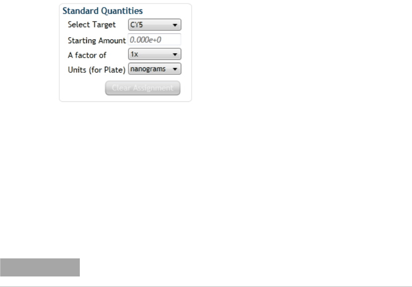
6 Setting Up the Plate
Assign plate properties for a User Defined experiment
141 Agilent Aria Real-Time PCR Program
Assign quantities to Standard wells
In order to generate a standard curve from your data, you need to assign
the initial template quantity to each Standard well.
To assign the standard quantities for a target in the Standard wells:
1 On the Plate Setup screen, select the Standard wells. (For instructions
on well selection, see “Select and view wells in the plate map” on
page 79.)
2 In the Properties panel under Standard Quantities, select which target
in the selected wells is the standard target (i.e., the target of known
quantity in the template).
3 In the Starting Amount field, type in the quantity of the standard target
present in the first replicate set of Standard wells. You will be asked to
specify the units for this amount step 5.
4 In the drop- down list labeled A factor of, select the dilution factor
used to generate the dilution series of the standard template. For
example, if each standard quantity is separated by a factor of 10, select
10x. Negative dilution factors are used to specify a decrease in quantity
from the starting amount while positive dilution factors specify an
increase from the starting amount.
5 In the drop- down list labeled Units (for Plate), select the units of the
quantity entered in the Starting Amount field. Note that all Standard
wells on the plate must use the same units.
To clear the assigned standard quantity from one or more wells:
• Select the well(s) and click Clear.
NOTE
This quantity must be either the highest quantity or the lowest quantity in the
dilution series of the standard template sample.

7 Setting Up the Thermal Profile
Set up the thermal profile
143 Agilent Aria Real-Time PCR Program
Set up the thermal profile
In the center of the Thermal Profile screen is a visual representation of
the temperature cycling program that directs the instrument to incubate
samples at specific temperatures for specific times.
To open the Thermal Profile screen: With an experiment or project file
open, click Thermal Profile in the Experiment Area panel on the left side
of the screen.
When you create a new experiment based on experiment type, a default
thermal profile is automatically assigned by the program. The default
thermal profile is one that is typical for the needs of that experiment
type. (The exception is User Defined experiments. Instead of assigning a
default thermal profile, the program prompts you to select a thermal
profile from a set of defaults). If you created the experiment from a
template, the default thermal profile is that of the template. You can also
import a thermal profile from an existing experiment (see “Import a
thermal profile” on page 146). In any pre- run experiment, you can edit
the thermal profile to fit your needs (see “Edit the thermal profile” on
page 147).

Setting Up the Thermal Profile 7
Set up the thermal profile
Agilent Aria Real-Time PCR Program 144
Elements of a Thermal Profile
Plateau
A plateau is a temperature held by the instrument for a specified
duration. It is represented with a solid horizontal line in the thermal
profile with the duration of the plateau displayed directly above the line
and the temperature of the plateau displayed directly below the line. The
valid range for a plateau duration is 1 second to greater than 18 hours.
The valid temperature range is 25.0° (ambient) to 99.9°C.
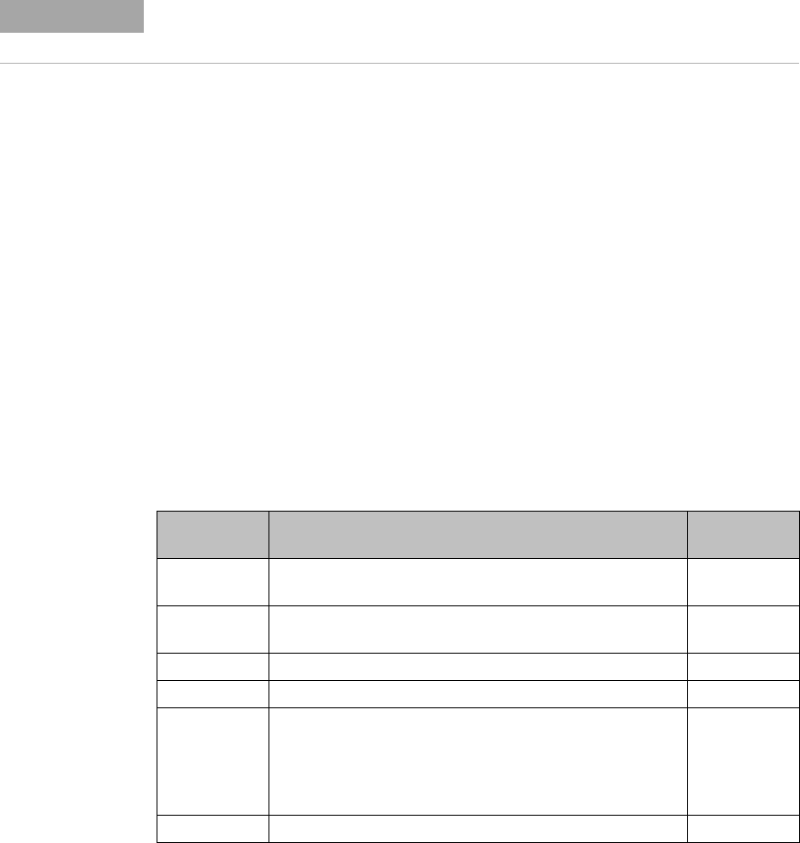
7 Setting Up the Thermal Profile
Set up the thermal profile
145 Agilent Aria Real-Time PCR Program
Ramp
A ramp is the transition between two plateaus. When you add a new
plateau to the thermal profile, the program automatically adds ramps
leading to and from the new plateau temperature. Likewise, when you
delete a segment or plateau, the program removes the associated ramps to
connect adjacent plateaus.
Segment and Number of Cycles
A segment is a group of plateaus and the intervening ramps that has been
set to cycle at least one time. Segments are delineated in the thermal
profile by solid vertical lines. A cycle is one pass through a segment. The
cycle number for the segment is displayed at the bottom of the thermal
profile.
The table below lists the types of segments and the maximum number of
cycles allowed for each segment type.
Table: Available segment types
* The thermal profile cannot include more than 5 segments that have >50 cycles.
NOTE
During plateaus with a temperature lower than 40°C, the heated lid of the thermal block
remains off, even when the instrument Hot Top Setting is enabled.
Segment Type Description Maximum # of
cycles
Amp. 2-Step Amplification using 2 plateaus: one for denaturation and one for
annealing/extension
255*
Amp. 3-Step Amplification using 3 plateaus: one for denaturation, one for
annealing, and one for extension
255*
Melt Melt/dissociation of PCR products 1
Hot Start Hot start activation of PCR enzyme 1
UDG (DNA) Uracil-DNA glycosylation reaction; in a reaction in which UNG
(uracil-N-glycosylase) was used to digest amplicon carryover
from a previous PCR amplification, you can add this segment to
the beginning of the thermal profile to heat inactivate the UNG
enzyme
1
RT Reverse transcription of RNA into DNA 1
Setting Up the Thermal Profile 7
Set up the thermal profile
Agilent Aria Real-Time PCR Program 146
Data Collection Marker
A data collection marker is a magnifying glass icon that indicates the
points designated for fluorescence data collection by the instrument. For
data collection markers on a plateau, the instrument collects fluorescence
data at the end of the plateau duration. The minimum duration for a
plateau that includes data collection is 3 seconds. For data collection
markers on a melt ramp (only melt segment ramps can accept collection
markers), the instrument collects fluorescence data throughout the ramp
period.
Touchdown Settings
Touchdown settings allow you to incrementally change the duration or
temperature of a plateau with each cycle within the segment. Touchdown
settings can be applied to a plateau in an amplification segment (see “Edit
touchdown settings (plateaus in amplification segments only)” on
page 152). When an amplification segment includes a plateau with
touchdown properties, the settings are displayed at the top of the segment
in the thermal profile.
Ramp Mode Settings
Ramp mode settings are applicable to melt segments that include data
collection (see “Edit ramp properties (melt segments only)” on page 154).
These settings include the resolution and soak time, and they are
displayed at the top of the melt segment in the thermal profile.
Import a thermal profile
From the Thermal Profile screen, you can import a thermal profile setup
from an existing pre- run or post- run experiment file or template file.
Once imported, you can edit the thermal profile as desired (see “Edit the
thermal profile” on page 147).
The experiment or template used for import must be the same experiment
type as the current experiment and have a valid thermal profile (review
“Elements of a Thermal Profile” on page 144 for information on
restrictions).
7 Setting Up the Thermal Profile
Set up the thermal profile
147 Agilent Aria Real-Time PCR Program
To import a thermal profile setup:
1 Right- click on the thermal profile display. In the menu that opens, click
Import Thermal Profile Setup.
The Open dialog box opens.
2 At the bottom of the dialog box, use the drop- down list to select the
appropriate file type (Experiment Files or Template Files).
3 Browse to the file from which you want to import the thermal profile
setup. Select the file and click Open. The software imports the thermal
profile into the experiment.
A message box opens notifying you that the import was successful.
4 Click OK in the message box to close it.
The thermal profile display is updated to the imported setup.
Edit the thermal profile
From the Thermal Profile screen, you can edit any element of the thermal
profile, including adding and deleting segments and plateaus and changing
plateau temperatures and durations.
Edit plateaus
To edit a plateau temperature:
1 In the display, click directly on the plateau temperature that you want
to edit.
The temperature becomes an editable field.
2 Type the desired temperature into the field, or click the +/- buttons
until you reach the desired temperature.
3 Press Enter, or click anywhere outside of the field.
You can also adjust plateau temperature by clicking on the plateau and
dragging it up or down to a new temperature.
To edit a plateau duration:
1 In the display, click directly on the plateau duration that you want to
edit (durations are displayed as minutes:seconds).
The duration becomes an editable field.
Setting Up the Thermal Profile 7
Set up the thermal profile
Agilent Aria Real-Time PCR Program 148
2 Type the desired duration for the plateau into the field, or click the +/-
buttons until you reach the desired duration.
When typing in the duration, you can either type the number of
seconds and let the program convert it to the minutes:seconds format
(e.g., an entry of “120” would be converted to “2:00”), or you can type
in the duration using the minutes:seconds format.
3 Press Enter, or click anywhere outside of the field.
To add a plateau:
1 On the display, locate the segment to which you want to add a plateau.
2 Within that segment, select the existing plateau that needs to precede
the new plateau. (To select a plateau, click directly on it. The plateau
becomes red in the display.)
If you need the new plateau to be the first plateau in the segment, skip
step 2 and go directly to step 3.
3 Right- click within the same segment.
A short- cut menu opens.
4 Click Add Plateau.
The program adds a new plateau immediately after the selected plateau
(or to the start of the segment if no plateau is selected). The new
plateau has a 25°C temperature and a 30- second duration. The program
allows up to 20 plateaus per segment and up to 150 total plateaus in a
thermal profile.
5 Edit the temperature and duration of the new plateau as needed. See
the instructions above (To edit a plateau temperature and To edit a
plateau duration).
To remove a plateau:
1 On the display, select the plateau that you want to remove. (To select a
plateau, click directly on it. The plateau becomes red in the display.)
2 Right- click on the segment containing the selected plateau.
A short- cut menu opens.
3 Click Remove Plateau.
The program deletes the selected plateau from the thermal profile.

7 Setting Up the Thermal Profile
Set up the thermal profile
149 Agilent Aria Real-Time PCR Program
Edit segments
To add a segment:
1 On the display, hover your cursor over an existing segment that will be
adjacent to the new segment.
2 Click the + icon (shown below) on either the left side or right side of
the existing segment.
Clicking the icon on the left adds the new segment just before the
existing segment. Clicking the icon on the right adds the new segment
just after the existing segment.
NOTE
For instructions on editing the touchdown properties of a plateau in an
amplification segment, see “Edit touchdown settings (plateaus in amplification
segments only)” on page 152.

Setting Up the Thermal Profile 7
Set up the thermal profile
Agilent Aria Real-Time PCR Program 150
The program opens a placeholder for the new segment (shown below)
listing the available segment types.
3 In the placeholder, click the type of segment that you want to add.
The program adds the new segment to the thermal profile. The program
allows up to 20 segments in a thermal profile.
Refer to the table in “Segment and Number of Cycles” for a description
of each available segment type.
4 Edit the plateaus or number of cycles for the segment as desired.
7 Setting Up the Thermal Profile
Set up the thermal profile
151 Agilent Aria Real-Time PCR Program
To remove a segment:
1 On the display, hover your cursor over the segment that you want to
remove.
An X appears at the top of the segment to the right of the segment
name.
2 Click the X.
The program deletes the segment from the thermal profile.
To move a segment:
1 Click and drag the segment that you want to move to the left or right.
The purple line indicates where in the thermal profile you have dragged
the segment.
2 When the purple line is in the desired location, release the left mouse
button to drop the segment into that position.
To change the number of steps in an amplification segment:
1 On the display, right- click on the amplification segment.
A short- cut menu opens.
2 If you want to change from a 3- step amplification to a 2- step
amplification, click Change to Amp. 2- Step. If you want to change from
a 2- step amplification to a 3- step amplification, click Change to Amp.
3- Step.
The program adjusts the number of plateaus in the thermal profile
according to your selection.
A 3- step amplification segment has 3 plateaus: one for denaturation,
one for annealing, and one for extension. A 2- step amplification
segment has only 2 plateaus: one for denaturation and a combined
annealing/extension plateau.
To change the number of cycles for an Amplification segment:
1 On the display, click directly on the number of cycles shown at the
bottom of the segment.
The cycle number becomes an editable field.
2 Type the desired number of cycles into the field, or click the +/-
buttons until you reach the desired number.
3 Press Enter, or click anywhere outside of the field.
Setting Up the Thermal Profile 7
Set up the thermal profile
Agilent Aria Real-Time PCR Program 152
Edit data collection markers
To add a data collection marker:
1 On the display, hover the cursor over the plateau or ramp where you
want to add a new data collection marker.
A grayed out image of a data collection marker appears on the display.
2 Click the image of the data collection marker.
The program adds the data collection marker to the thermal profile.
Only melt segments can have a data collection marker assigned to a
ramp.
You can add up to 20 data collection markers to an amplification
segment.
To remove a data collection marker:
• On the display, click directly on the data collection marker that you
want to remove.
The program removes the data collection marker from the thermal
profile.
Edit touchdown settings (plateaus in amplification segments only)
1 On the display, locate the amplification segment that contains the
plateau to be edited. Make sure that the segment has already been
assigned the desired number of cycles.
The number of cycles assigned to the segment impacts the touchdown
settings. See the note, Best practices for touchdown PCR.
2 Select the desired plateau within the amplification segment. (To select a
plateau, click directly on it. The plateau becomes red in the display.)
3 Right- click on the segment containing the selected plateau.
A short- cut menu opens.
4 Click Touchdown Settings.

7 Setting Up the Thermal Profile
Set up the thermal profile
153 Agilent Aria Real-Time PCR Program
The Touchdown Settings dialog box opens.
5 In the Time Step (mm:ss) field, add an increment to the duration of
the plateau. The permitted range for the selected plateau (called the
Valid Time Range) is displayed near the bottom of the Touchdown
Settings dialog box. This range is based on the initial duration of the
plateau and the number of cycles assigned to the segment. The
maximum value for the range is designed to ensure that by the last
cycle, the duration of the plateau does not exceed the maximum
allowed duration.
During the run, the duration of the plateau increases with each cycle by
the specified number of minutes and seconds (mm:ss). For example,
enter a Time Step of 00:05 to increase the duration of the plateau by
an additional 5 seconds with each cycle.
6 In the Temperature Step (°C) field, add an increment to the
temperature of the plateau. The permitted range for the selected
plateau (called the Valid Temperature Range) is displayed near the
bottom of the Touchdown Settings dialog box. This range is based on
the initial temperature of the plateau and the number of cycles assigned
to the segment. The range values are designed to ensure that by the last
cycle, the temperature of the plateau does not exceed the maximum
allowed temperature of 99.9°C, or fall below the minimum allowed
temperature of 25°C.
During the run, the temperature of the plateau increases (for positive
numbers) or decreases (for negative numbers) with each cycle by the
specified number of degrees. For example, enter a Temperature Step of
–0.5 to decrease the temperature of the plateau by 0.5°C with each
cycle.

Setting Up the Thermal Profile 7
Set up the thermal profile
Agilent Aria Real-Time PCR Program 154
7 Click OK to close the dialog box and save your changes.
Edit ramp properties (melt segments only)
If you are collecting data during a ramp within a melt or high resolution
melt segment, you can edit the resolution and the soak time. The
Best practices for touchdown PCR
If touchdown PCR is only required until a particular plateau duration or plateau temp-
erature is reached, set up the thermal profile to include two amplification segments, and
only program the first amplification segment to include touchdown settings. For example,
if the desired thermal profile has 40 amplification cycles, with an initial annealing
temperature of 70°C and a final annealing temperature of 60°C, include two amplification
segments in the thermal profile. In the first amplification segment, set the segment to
cycle 10 times. Include an annealing plateau of 70°C, and to this plateau, add touchdown
PCR settings with a temperature step of -1°C so that the plateau temperature is 61°C
during the 10th cycle. In the second amplification segment, set the segment to cycle 30
times. Include an annealing plateau of 60°C and do not add any touchdown PCR settings.

7 Setting Up the Thermal Profile
Set up the thermal profile
155 Agilent Aria Real-Time PCR Program
resolution sets the temperature increments of the ramp. The soak time is
the length of time that the instrument holds each incremental temperature
during the ramp.
To change the resolution of a ramp:
1 On the melt segment, click the area below the segment name that
displays the resolution and soak time.
The Ramp Mode dialog box opens.
2 Next to Resolution (°C), select 0.2 to set the ramp to 0.2°C increments,
or select 0.5 to set the ramp to 0.5°C increments.
A resolution of 0.2 yields a high resolution melt curve.
3 Click OK to close the dialog box and save your changes.
Melt segments with a resolution of 0.2 are named High Resolution Melt.
Melt segments with a resolution of 0.5 are named Melt.
NOTE
Melt segments can have only one data collection marker.
You can only change the ramp resolution if the experiment is an Allele
Discrimination - DNA Binding Dye experiment or a User Defined experiment.

Setting Up the Thermal Profile 7
Set up the thermal profile
Agilent Aria Real-Time PCR Program 156
To change the soak time for a ramp:
1 On the melt segment, click the area below the segment name that
displays the resolution and soak time.
The Ramp Mode dialog box opens.
2 Next to Soak Time, type in the desired number of seconds for the soak
time, or click the +/- buttons to adjust the value in the field.
The soak time is the amount of time that the instrument spends at each
temperature increment during the ramp.
3 Click OK to close the dialog box and save your changes.
Restore the default thermal profile
To restore the thermal profile to the default for the experiment type:
1 Right- click anywhere on the thermal profile display.
A short- cut menu opens.
2 Click Restore Default Thermal Profile.
The program sets the thermal profile to the default for the experiment
type.
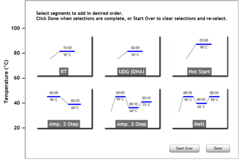
7 Setting Up the Thermal Profile
Set up the thermal profile
157 Agilent Aria Real-Time PCR Program
Select segments for a blank thermal profile
If you delete all segments in a thermal profile, or if you create a new User
Defined experiment, the thermal profile screen appears as shown below.
On this screen, you select the segments you want to use to create a new
thermal profile.
To select segments to add to a blank thermal profile:
1 From the screen shown above, click on the segment type that you want
to be the first segment in the thermal profile.
The program marks the segment with a number “1” in the upper left
corner, as in the example image shown below.

Setting Up the Thermal Profile 7
Set up the thermal profile
Agilent Aria Real-Time PCR Program 158
2 Click on the segment type that you want to be the second segment in
the thermal profile.
The program marks the segment with a number “2” in the upper left
corner.
3 Continue clicking on segments to build the thermal profile. If you need
to redo an assignment, click Start Over. When finished building the
thermal profile click Done.
The program generates the thermal profile based on your selections and
displays it on the Thermal Profile screen.
4 Edit the thermal profile as needed.
7 Setting Up the Thermal Profile
Export the thermal profile image
159 Agilent Aria Real-Time PCR Program
Export the thermal profile image
The image of the thermal profile can be exported to a Microsoft
PowerPoint presentation.
To export an image of the thermal profile to PowerPoint:
• From the Thermal Profile screen, right click anywhere on the display.
In the short- cut menu, click Send Image to PowerPoint.
PowerPoint opens to a new presentation file with the thermal profile
image on the slide.

Agilent Technologies
8
Running and Monitoring Experiments
Overview of the Instrument Explorer dialog box 161
Add instruments to your network 162
Add a new instrument based on its IP address 162
Add a new instrument based on its port number 163
View information about an instrument 163
Start, stop, or pause a run 165
Start a run 165
Cancel a run 166
Pause a run 167
Monitor a run 168
Connect to the running instrument 168
Monitor a run by viewing its progress through the thermal profile 169
Monitor a run by viewing the raw data plots 169
Change the display options for the raw data plots 170
Stop monitoring a run 172
Retrieve run data from the instrument 173
Retrieve data through the network 173
Retrieve data using a USB drive 174
Export instrument data to a CSV file 175
Export instrument data by column 175
Export instrument data by target 175
Export instrument data by wells 175
8 Running and Monitoring Experiments
Overview of the Instrument Explorer dialog box
161 Agilent Aria Real-Time PCR Program
Overview of the Instrument Explorer dialog box
The Instrument Explorer dialog box has tools for performing a variety of
functions that require connecting to an instrument through a local
network.
To open the Instrument Explorer dialog box:
• For starting and monitoring a run, open the Thermal Profile, Run
Status, or Raw Data Plots screen and click Run.
• For other Instrument Explorer functions, at the top of the program
window, click Instrument > Instrument Explorer. (Starting a run is not
enabled when you open the dialog box from the Instrument menu.
However, opening the dialog box from the Instrument menu does allow
you to monitor a run that has already been started.)
See the following help topics for instructions on specific tasks that require
the use of the Instrument Explorer dialog box.
“Add instruments to your network” on page 162
“Start, stop, or pause a run” on page 165
“Monitor a run” on page 168
“Retrieve run data from the instrument” on page 173
“Export instrument data to a CSV file” on page 175

Running and Monitoring Experiments 8
Add instruments to your network
Agilent Aria Real-Time PCR Program 162
Add instruments to your network
The Instrument Explorer dialog box lists the instruments connected to
your subnetwork. If the instrument you need is not displayed in the list,
the dialog box has tools to search for and add a new instrument.
To open the Instrument Explorer dialog box: At the top of the program
window, click Instrument > Instrument Explorer. (Note that in order to
start a run, you must open the dialog box by clicking Run on the Thermal
Profile, Run Status, or Raw Data Plots screen. Starting a run is not
enabled when you open the dialog box from the Instrument menu.
However, opening the dialog box from the Instrument menu does allow you
to monitor a run that has already been started.)
Add a new instrument based on its IP address
If you do not see the instrument you are looking for listed on the
Instrument Explorer dialog box, you can search for and add an instrument
by its IP address.
To search for and connect to an instrument based on its IP address:
1 In the Instrument Explorer dialog box, click the Add Instrument icon.
The Add Instrument dialog box opens.
2 In the Instrument field, type the IP address of the instrument you want
to connect to, then click Add.
The Add Instrument dialog box closes and the instrument is listed in
the Instrument Explorer dialog box.
NOTE
You can look up the IP address of an instrument through the touchscreen. Near
the bottom right corner of the Home screen, press the Connections button (shown
below). The pop-up box that opens includes the instrument's IP address.

8 Running and Monitoring Experiments
Add instruments to your network
163 Agilent Aria Real-Time PCR Program
Add a new instrument based on its port number
If you do not see the instrument you are looking for listed on the
Instrument Explorer dialog box, you can search for and add instruments
that are connected to the network on a different port number.
To select port numbers on which the application searches for available
instruments:
1 In the Instrument Explorer dialog box, click the Discovery Port icon,
The Discovery Port dialog box opens. The marked port numbers are the
ones on which the program currently searches for instruments.
2 Mark the port number you want to search.
• If the port number is already listed in the Discovery Port dialog box,
mark the check box in the Use column.
• If the port number is not listed, click the Add icon to add
additional ports.
• For any listed ports that you do not want included in the search,
clear the check box next to the port number or select the port
number and click the Delete icon .
3 Click OK to save your changes and close the Discovery Port dialog box.
The instruments from the selected port number are listed in the
Instrument Explorer dialog box.
View information about an instrument
For the available instruments listed in the Instrument Explorer dialog box,
you can view information about the instrument including:
• The optical modules that are installed on the instrument
• The instrument serial number
• The IP address for the instrument
• The firmware version installed on the instrument

Running and Monitoring Experiments 8
Add instruments to your network
Agilent Aria Real-Time PCR Program 164
To view instrument information:
1 In the Instrument Explorer dialog box, click the Instrument Information
icon next to the desired instrument.
The Instrument Information dialog box opens.
8 Running and Monitoring Experiments
Start, stop, or pause a run
165 Agilent Aria Real-Time PCR Program
Start, stop, or pause a run
Starting a run causes the instrument to initiate the thermal profile
protocol.
Start a run
To start running an experiment:
1 Set up the experiment in the program (either using the PC version of
the Aria program or using the touchscreen program) and set up the
PCR reactions in the 96- well reaction plate.
Setting up the experiment in the software requires creating the
experiment file, setting up the plate and, setting up the thermal profile.
2 Start the run:
• If you are working from the PC version of the program:
a Open the Thermal Profile screen, Run Status screen, or Raw Data
Plots screen.
b Click Run.
The Instrument Explorer dialog box opens.
If the open experiment is a post- run experiment, you will first be
prompted to save the experiment with a new name.
c Locate the instrument that you will be using for the run and click
Send Config. (See “Add instruments to your network” on page 162
for instructions on searching for and adding instruments.)
• If this is the first time you have connected to an instrument
since last launching the Aria program, the Login dialog box
opens. Select your Username from the drop- down list, type
your login password into the Password field, and click Login.
To log in with a different user account, right- click on the
instrument name and click Log off current user. You can then
log in using the desired user account.
• If the experiment is new, you will be prompted to save the
experiment before proceeding.
d Take your reaction plate over to the instrument and load it into
the thermal block.
Running and Monitoring Experiments 8
Start, stop, or pause a run
Agilent Aria Real-Time PCR Program 166
e On the instrument touchscreen, open the primed experiment to the
Thermal Profile screen and press Run Experiment.The instrument
starts running the experiment.
f Return to the PC program. The program directs you to the Run
Status screen, where you can monitor the progress of the run. See
“Monitor a run” on page 168.
• If you are working from the touchscreen version of the program:
a Load your reaction plate into the instrument's thermal block.
b On the Thermal Profile screen, press Run Experiment.
The instrument starts running the experiment. You can monitor
the progress of the run from your PC. See “Monitor a run” on
page 168 for instructions.
Cancel a run
To stop an in- progress run:
1 Make sure you are monitoring the run. See “Monitor a run” on
page 168.
2 On the Run Status or Raw Data Plots screen, click Stop Run.
A message box opens asking you to confirm that you want to stop the
run.
3 In the message box, if you do not want to save the partial data
collected during the run, mark the check box labeled Discard
Instrument Data. If you do want to save the partial data, leave the
check box unmarked.
4 Click Abort Experiment in the message box to stop the run.
If you chose to save the partial data, you can view it on the Graphical
Displays screen.
8 Running and Monitoring Experiments
Start, stop, or pause a run
167 Agilent Aria Real-Time PCR Program
Pause a run
To pause an in- progress run:
1 Make sure you are monitoring the run. See “Monitor a run” on
page 168.
2 On the Run Status or Raw Data Plots screen, click Pause.
A message box opens asking you to confirm that you want to pause the
run.
3 In the message box, click Pause Run.
The program pauses the run. When you are ready to resume running
the experiment, click Resume.

Running and Monitoring Experiments 8
Monitor a run
Agilent Aria Real-Time PCR Program 168
Monitor a run
The Run Status and Raw Data Plots screens allow you to start a run and
to monitor the progress of a run. The Run Status screen shows the
progression of the run through the thermal profile. The Raw Data Plots
screen displays the amplification or melt data in each well as it is
collected by the instrument in real- time.
To open the Run Status or Raw Data Plots screen: Click Run Status or
Raw Data Plots in the Experiment Area panel on the left side of the
screen.
Connect to the running instrument
To connect to the instrument that is running the experiment that you
want to monitor:
1 At the top of the program window, click Instrument > Instrument
Explorer.
2 Locate the instrument and click Monitor Run. (If the instrument is not
listed, see “Add instruments to your network” on page 162 for
instructions on searching for and adding instruments.)
If this is the first time you have connected to an instrument since last
launching the Aria program, the Login dialog box opens. Select your
Username from the drop- down list, type your login password into the
Password field, and click Login.
NOTE
Only one computer can monitor the run on a particular instrument at any one time.
If you are monitoring a run when the run completes, the instrument will
automatically transfer the run data to the PC, unless you logged into the
instrument using the guest account. If you logged in as guest, you must retrieve
the data in order to view the results on your PC. See “Retrieve run data from the
instrument” on page 173 for more information.
If you are monitoring a run, and someone stops the run from the instrument
touchscreen, the program opens a message notifying you that the run has been
stopped. The message will indicate whether or not the user who stopped the run
selected to save the partial data from the run. If partial data was saved, you will
need to retrieve it. See “Retrieve run data from the instrument” on page 173.
8 Running and Monitoring Experiments
Monitor a run
169 Agilent Aria Real-Time PCR Program
The program directs you to the Run Status screen.
Monitor a run by viewing its progress through the thermal profile
The Run Status screen allows you to monitor a run by viewing the
instrument's progress through the thermal profile of the experiment.
To monitor the run status:
1 Connect to the running instrument.
2 Open the Run Status screen.
In the center of the screen is a representation of the thermal profile for
the experiment. As an experiment is running, the progression of the
experiment through the thermal profile protocol is indicated on the
display.
The top of the screen lists the time remaining in the run and the
current temperature. The bottom of each segment shows how many
cycles of the segment have been completed.
Monitor a run by viewing the raw data plots
The Raw Data Plots screen allows you to monitor a run by watching the
real- time changes in fluorescence levels in the individual wells. The
program displays these changes as raw data plots, which are graphs that
plot the fluorescence values on the Y- axis in relative fluorescence units
(RFU).
To monitor the raw data plots:
1 Connect to the running instrument.
2 Open the Raw Data Plots screen.
On the left side of the screen is a representation of the experiment
plate. During the run, the raw data are plotted and displayed in each
well. The Y- axis of the plots shows the level of raw fluorescence. If
monitoring data collection for an Amplification segment, the X- axis
plots the cycle number. If monitoring data collection for a melt segment,
the X- axis plots the temperature.

Running and Monitoring Experiments 8
Monitor a run
Agilent Aria Real-Time PCR Program 170
On the right side of the screen is an expanded view of the raw data
plots within a selected well or a set of selected wells. Hover your cursor
over any individual plot line in this view to see which well and target
that line refers to. Hover your cursor over a well on the plate to
highlight the plot line for that well in the raw data plots.
Change the display options for the raw data plots
Change which data collection marker is used for the plots
By default, the raw data plots show the data collected during the
amplification segment of the thermal profile.
To select a different data collection marker to display in the raw data
plots:
1 On the Raw Data Plots screen, hover your cursor over the Data
Collection Marker icon at the bottom of the screen.
A window opens displaying the thermal profile with data collection
markers.
2 Click the data collection marker that you want to use for the raw data
plots.
The window closes and the program uses the selected data collection
marker in the raw data plots.
Select which targets to include in the plots
By default, the raw data for all targets in use on the plate are included in
the plots.
To select specific targets to display in the raw data plots:
1 On the Raw Data Plots screen, hover your cursor over the Display
Targets icon at the bottom of the screen.
A window opens showing all targets in use on the plate.

8 Running and Monitoring Experiments
Monitor a run
171 Agilent Aria Real-Time PCR Program
2 For any targets that you do not want displayed, clear the check box
next to the target name. You can remark the check box at any time to
add the target back to the raw data plots.
Select which well types to include
By default, the raw data plots are displayed for all well types in use on
the plate.
To show the raw data for only specific well types:
1 On the Raw Data Plots screen, hover your cursor over the Display Well
Types icon at the bottom of the screen.
A window opens showing all well types in use on the plate.
2 For any well types that you do not want to include, clear the check box
next to the well type name. You can remark the check box at any time
to add the well type back to the raw data plots.
Change the scale or orientation of the axes
By default, the X and Y axes of the graph on the right side of the Raw
Data Plots screen are oriented in ascending order and the ranges of the
axes adjust automatically based on the plots being displayed.
To change the orientation of the X or Y axis:
1 Right- click anywhere on the large graph of the Raw Data Plots screen.
A short- cut menu opens.
2 Click Axis Options > Reverse Orientation in X- Axis or Axis Options >
Reverse Orientation of Y- Axis.
The program reverse the orientation of the selected axis.
To change the scale of the X or Y axis:
1 Right- click anywhere on the large graph of the Raw Data Plots screen.
A short- cut menu opens.
2 Click Axis Options > Customize Scale.
The Graph Properties dialog box opens to the Axis Options tab.
Running and Monitoring Experiments 8
Monitor a run
Agilent Aria Real-Time PCR Program 172
3 Under the heading for the desired axis, change the Autoscale setting to
Manual.
4 In the Min and Max fields, type the desired minimum and maximum
values for the scale of the axis.
5 Click Close to save your changes and close the Graph Properties dialog
box.
The program sets the scale of the axis to the new values.
Stop monitoring a run
When you stop monitoring a run, the instrument continues running the
experiment and the run becomes available for monitoring from another
PC.
To stop monitoring a run, do one of the following:
• Close the experiment.
• From the Run Status or Raw Data Plots screen, click Stop Monitor. In
the message box that opens, click Yes to confirm that you want to stop
monitoring the run.

8 Running and Monitoring Experiments
Retrieve run data from the instrument
173 Agilent Aria Real-Time PCR Program
Retrieve run data from the instrument
If you are monitoring a run from your PC when the run completes, the
instrument will automatically transfer the run data to the PC program
(unless you logged into the instrument using the guest account). If you are
not monitoring the run, the data from the run is saved to the instrument
and you must retrieve it to your PC in order to analyze the experiment
results. You can retrieve the data through the network, or by copying it to
a USB drive.
Retrieve data through the network
If the instrument is connected to the same network as your PC, you can
retrieve data by connecting to the instrument remotely.
To retrieve the data from a run by remotely connecting to the instrument
from your PC:
1 Make sure the experiment file is not open on the instrument.
2 From your PC, click Instrument > Instrument Explorer.
The Instrument Explorer dialog box opens.
3 Locate the instrument on which you ran the experiment, and in that
row, click the File Explorer icon.
The File Explorer dialog box opens.
If this is the first time you have connected to an instrument since last
launching the application, the Login dialog box opens. Select your
Username from the drop- down list, type your login password into the
Password field, and click Login. After logging in, the File Explorer
dialog box opens.
4 In the list of folders on the left side of the File Explorer dialog box,
browse to the folder of the experiment on the instrument.
The root folder for the experiment is the folder for the user who ran
the experiment. The subfolder is named for the experiment type.
5 Click directly on the experiment for which you want to transfer the run
data.
6 Click Copy & Delete.
Running and Monitoring Experiments 8
Retrieve run data from the instrument
Agilent Aria Real-Time PCR Program 174
The program transfers the post- run experiment file from the instrument
to the default experiment storage folder on your PC (the program
deletes the file from the instrument in the process). If the pre- run
experiment is already saved to your PC, the program saves the post- run
experiment file with a bracketed number appended to the end of the
file name (e.g., Experiment1[1]).
7 Open the experiment file in the Aria program to view the results of the
run.
Retrieve data using a USB drive
You can connect a USB drive to the instrument and save the data to the
drive, and then transfer it to your PC. This approach is the only way to
retrieve data from an instrument that is not network- connected.
1 Insert an external USB drive (FAT format) into the USB port on the
front of the instrument.
2 On the instrument touchscreen, open the folder with the post- run
experiment file.
3 Copy the experiment to the USB drive.
After successful transfer of the file, delete the file from the instrument
to avoid filling the instrument's hard drive.
4 Remove the USB drive from the instrument and insert it into your PC.
5 Move the experiment file to a folder of your choice.
6 Open the experiment file in the Aria program to view the results of the
run.
8 Running and Monitoring Experiments
Export instrument data to a CSV file
175 Agilent Aria Real-Time PCR Program
Export instrument data to a CSV file
For each post- run experiment, the program stores the raw data for all
dyes in all wells at each data collection point. To view this data, export it
to a CSV file and then open it in Excel.
Export instrument data by column
To export instrument data by column:
1 Click Instrument > Export Instrument Data > By Columns.
The Export Instrument Data By Columns dialog box opens.
2 Select a folder and file name for the CSV file and click Save.
The program generates the file and opens it in Microsoft Excel.
Export instrument data by target
To export instrument data by target:
1 Click Instrument > Export Instrument Data > By Target.
The Export Instrument Data By Target dialog box opens.
2 Select a folder and file name for the CSV file and click Save.
The program generates the file and opens it in Microsoft Excel.
Export instrument data by wells
To export instrument data by wells:
1 Click Instrument > Export Instrument Data > By Wells.
The Export Instrument Data By Wells dialog box opens.
2 Select a folder and file name for the CSV file and click Save.
The program generates the file and opens it in Microsoft Excel.

Agilent Technologies
9
Setting Analysis Criteria
Overview of the Analysis Criteria screen 177
Toggle display of plate map wells 178
Select the wells and well types to include in analysis 179
Select wells for analysis using the plate map 179
Select wells for analysis based on well type 179
Select the targets to include in analysis 180
Select which data collection points to analyze 181
Choose a treatment for replicate wells 182
Assign an HRM calibration plate 183
Assign an HCP for new experiments 183
Assign an HCP using the HCP icon 184

9 Setting Analysis Criteria
Overview of the Analysis Criteria screen
177 Agilent Aria Real-Time PCR Program
Overview of the Analysis Criteria screen
Your selections on the Analysis Criteria screen determine the settings that
the program uses for data analysis.
To open the Analysis Criteria screen: Click Analysis Criteria in the
Experiment Area panel on the left side of the screen.
The Analysis Criteria screen has an image of the plate map that is based
on the settings on the Plate Setup screen. At the bottom of the screen are
icons that provide access to menus for making selections on which data
you want included in the results. Results are displayed on the Graphical
Displays screen.
See the following help topics for instructions on specific tasks for setting
the analysis criteria:
“Select the wells and well types to include in analysis” on page 179
“Select the targets to include in analysis” on page 180
“Select which data collection points to analyze” on page 181
“Choose a treatment for replicate wells” on page 182
“Assign an HRM calibration plate” on page 183 (only for experiments with
HRM segment)
Note that if you wish to use the default analysis settings, you need only
select the wells to analyze.
NOTE
The Analysis Criteria screen is only available in post-run experiments and
in-progress experiments that have completed at least one point of data collection.

Setting Analysis Criteria 9
Toggle display of plate map wells
Agilent Aria Real-Time PCR Program 178
Toggle display of plate map wells
The plate map on the Analysis Criteria screen can display either the
dye/target information and replicate number in each well, or it can display
the Cq value(s) calculated in each well. Your selection does not impact the
results shown on the Graphical Displays screen.
To open the Analysis Criteria screen: Click Analysis Criteria in the
Experiment Area panel on the left side of the screen.
To toggle between the two display options for the plate map on the
Analysis Criteria screen:
1 On the Analysis Criteria screen, click the Display toggle button at the
bottom of the screen. When the button looks like the image on the left,
the program is displaying the dye/target information and replicate
number in each well. When the button looks like the image on the right,
the program is displaying the Cq value(s) calculated in each well.

9 Setting Analysis Criteria
Select the wells and well types to include in analysis
179 Agilent Aria Real-Time PCR Program
Select the wells and well types to include in analysis
From the Analysis Criteria screen, you can select which wells and well
types to include in the results displayed on the Graphical Displays screen.
To open the Analysis Criteria screen: Click Analysis Criteria in the
Experiment Area panel on the left side of the screen.
Select wells for analysis using the plate map
The program's analysis algorithms only use the wells that are selected in
the plate map on the Analysis Criteria screen.
Well selection on the Analysis Criteria screen works that same way as it
does on the Plate Setup screen. See “Select wells in the plate map” on
page 79 for instructions on well selection.
Select wells for analysis based on well type
You can select specific wells to include in the analysis based on well type.
To select specific well types:
1 On the Analysis Criteria screen, hover your cursor over the Display Well
Types icon at the bottom of the screen.
A window opens showing all well types in use on the plate.
2 For any well types that you do not want to include, clear the check box
next to the well type name. You can remark the check box at any time
to reselect those wells.

Setting Analysis Criteria 9
Select the targets to include in analysis
Agilent Aria Real-Time PCR Program 180
Select the targets to include in analysis
From the Analysis Criteria screen, or from the Graphical Displays screen,
you can select which targets to include in the results displayed on the
Graphical Displays screen.
To open the Analysis Criteria screen: Click Analysis Criteria in the
Experiment Area panel on the left side of the screen.
To select specific targets:
1 On the Analysis Criteria screen, hover your cursor over the Display
Targets icon at the bottom of the screen.
A window opens showing all targets in use on the plate.
2 For any targets that you do not want included in the analysis, clear the
check box next to the target name. You can remark the check box at
any time to reselect those targets.

9 Setting Analysis Criteria
Select which data collection points to analyze
181 Agilent Aria Real-Time PCR Program
Select which data collection points to analyze
If your thermal profile includes multiple amplification collection points or
multiple melt collection points, you can specify on the Analysis Criteria
screen, or on the Graphical Displays screen, which data collection point to
use for analysis.
To open the Analysis Criteria screen: Click Analysis Criteria in the
Experiment Area panel on the left side of the screen.
To select which data collection point to use for analysis of amplification
data:
1 On the Analysis Criteria screen, hover your cursor over the Data
Collection Marker icon at the bottom of the screen.
A window opens displaying the thermal profile with data collection
markers.
2 Click the data collection marker within an amplification segment that
you want to use for analysis of amplification data.
The window closes and the program uses the selected data collection
marker to analyze amplification data.
To select which data collection point to use for analysis of melt data:
1 On the Analysis Criteria screen, hover your cursor over the Data
Collection Marker icon at the bottom of the screen.
A window opens displaying the thermal profile with data collection
markers.
2 Click the data collection marker within a melt segment that you want to
use for analysis of melt data.
The window closes and the program uses the selected data collection
marker to analyze melt data.

Setting Analysis Criteria 9
Choose a treatment for replicate wells
Agilent Aria Real-Time PCR Program 182
Choose a treatment for replicate wells
Data from wells identified as replicates in the plate setup can be treated
either individually (each well separate) or collectively (replicate wells
averaged at each cycle) during analysis. You can choose a treatment for
replicate wells from the Analysis Criteria screen, or from the Graphical
Displays screen.
To open the Analysis Criteria screen: Click Analysis Criteria in the
Experiment Area panel on the left side of the screen.
To specify that replicates be treated individually or collectively:
• On the Analysis Criteria screen, click the Replicates toggle button at the
bottom of the screen.
When the button looks like the image on the left, the program treats
them individually. When the button looks like the image on the right,
the program treats them collectively.
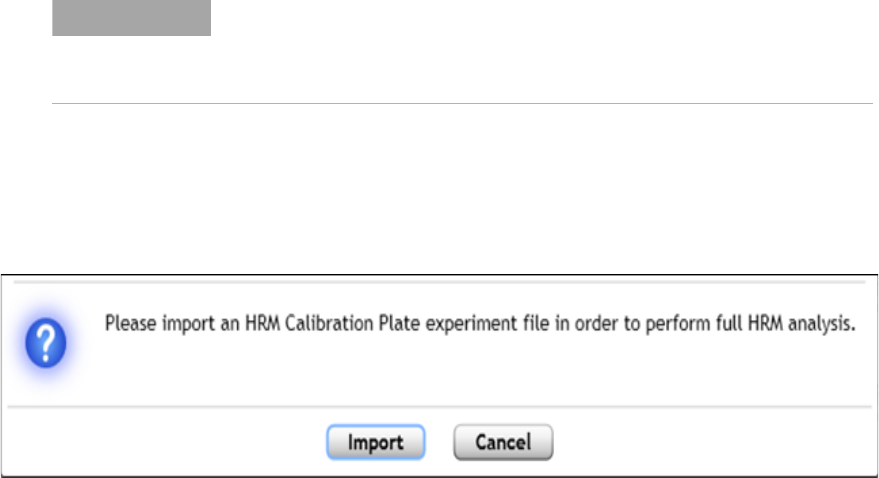
9 Setting Analysis Criteria
Assign an HRM calibration plate
183 Agilent Aria Real-Time PCR Program
Assign an HRM calibration plate
For an experiment that includes a high resolution melt (HRM) segment, in
order to view the Melt Curve - Difference Plots graph, the program
requires you to assign an HRM calibration plate (HCP) to the experiment.
In order to assign an HCP to an experiment, the HCP must:
• pass the system's quality check
• be run on the same instrument as your experiment with the HRM
segment
• have an identical soak time and plateau time in the HRM segment as
the experiment
Assign an HCP for new experiments
The first time you attempt to open the Analysis Criteria or Graphical
Displays screen for a new post- run experiment that includes an HRM
segment, the following message box opens on your screen.
To assign an HCP from the message box:
1 In the message box, click Import.
The Open dialog box opens.
2 Browse to the HCP file that you want to assign. Select the file and click
Open.
NOTE
A separate HRM software license is required in order to assign an HCP. To
purchase a software license, contact your Agilent Sales representative. The HRM
license option is only available for the AriaMx system. The license is not
supported for the AriaDx system.

Setting Analysis Criteria 9
Assign an HRM calibration plate
Agilent Aria Real-Time PCR Program 184
The program assigns the HCP to the experiment and calibrates the melt
data accordingly.
If you click Cancel in the message box shown above, you can still assign
an HCP using the HCP icon on the Analysis Criteria or Graphical Displays
screen. See instructions below.
Assign an HCP using the HCP icon
The HCP icon is available on the Analysis Criteria and Graphical Displays
screens for all experiments that include an HRM segment.
To assign an HCP:
1 On the Analysis Criteria or Graphical Displays screen, click the HCP
icon at the bottom of the screen.
The Open dialog box opens.
2 Browse to the HCP file that you want to assign. Select the file and click
Open.
The program assigns the HCP to the experiment and calibrates the melt
data accordingly.
To assign a recently used HCP:
1 On the Analysis Criteria or Graphical Displays screen, click the
arrowhead next to the HCP icon at the bottom of the screen.
2 In the menu that opens, hover your cursor over Recently Used Data.
A list of recently used HCPs opens.
3 Click the HCP that you want to assign to the current experiment.
The program assigns the HCP to the experiment and calibrates the melt
data accordingly.

9 Setting Analysis Criteria
Assign an HRM calibration plate
185 Agilent Aria Real-Time PCR Program
To clear an HCP assignment:
1 On the Analysis Criteria or Graphical Displays screen, click the
arrowhead next to the HCP icon at the bottom of the screen.
2 In the menu that opens, click Clear Calibration Data.
The experiment no longer has an HCP assigned. If desired, you can now
assign a different HCP to the experiment.

Agilent Technologies
10
Viewing Graphical Displays of the
Results
Overview of the Graphical Displays screen 187
Graphs 187
Result table 188
Display options 188
Zooming 190
Configure and apply analysis templates 192
Configure an analysis template in the Analysis Term Settings dialog
box 193
View the Amplification Plots 197
View the Melt Curve - Raw/Derivative Curve 212
View the Melt Curve - Difference Plots 218
View the Standard Curve 225
View the Relative Quantity 230
View the Allele Determination graph 235
Customize graph properties 240
Customize graph properties using the short-cut menu 240
Customize graph properties using the Graph Properties dialog
box 243

10 Viewing Graphical Displays of the Results
Overview of the Graphical Displays screen
187 Agilent Aria Real-Time PCR Program
Overview of the Graphical Displays screen
The Graphical Displays screen shows the results of the experiment
displayed in a series of graphs. For each graph, the screen includes tools
for setting certain analysis parameters. The screen also includes a result
table, with configurable columns of data, that you can export to an Excel
spreadsheet.
To open the Graphical Displays screen: Click Graphical Displays in the
Experiment Area panel on the left side of the screen.
Graphs
The exact set of graphs available on the Graphical Displays screen varies
depending on the experiment type, but all experiments have a graph of
the amplification plots, and all experiments with a melt segment have a
graph of the melt curves.
See the topics below for detailed information on specific graphs:
“View the Amplification Plots” on page 197
“View the Melt Curve - Raw/Derivative Curve” on page 212
“View the Melt Curve - Difference Plots” on page 218
“View the Standard Curve” on page 225
“View the Relative Quantity” on page 230
“View the Allele Determination graph” on page 235
By default, data from all of the wells that you selected on the Analysis
Criteria screen are displayed in the graphs. You can limit the graphs to
only display data from particular wells or replicate sets by selecting
specific rows in the result table (press Ctrl to select multiple rows). The
result table is described below.
NOTE
The Graphical Displays screen is only available in post-run experiments and
in-progress experiments that have completed at least one point of data collection.

Viewing Graphical Displays of the Results 10
Overview of the Graphical Displays screen
Agilent Aria Real-Time PCR Program 188
Result table
The result table on the right side of the Graphical Displays screen shows
results for each well (if replicates are treated individually) or replicate set
(if replicates are treated collectively) that you selected on the Analysis
Criteria screen (see “Select the wells and well types to include in analysis”
on page 179).
Row selection
You can select individual rows within the results table to limit the graphs
to displaying data only from particular wells/replicate sets. Click directly
on a row to select it. Press Ctrl to select multiple rows. By default, all
rows are initially selected. Click the Select All icon at the top of the
result table to reselect all rows.
Data columns
You can configure which columns of data are included in the table. Click
the Column Options icon at the top of the result table to open the
Column Options dialog box. In the dialog box, mark the columns that you
want to include in the result table.
You can freeze one or more columns on the left side of the result table so
that as you scroll through the table horizontally, the frozen columns are
always visible. Right- click on the header of the right- most column that
you want to freeze and click Freeze Column. To unfreeze, right- click
again and click Unfreeze Column.
Sorting
You can sort the data in the result table. Click directly on the header of
the column on which you want to sort. To designate a second column for
secondary sorting, press Shift then click the header of the second column.
The column headers selected for sorting are highlighted in blue.
Display options
When you have multiple graphs selected for viewing on the Graphical
Displays screen, you can manually drag and drop the graphs to new
positions on the screen using your cursor (the Manual Arrange feature).
Alternatively, you can select for the program to automatically arrange the

10 Viewing Graphical Displays of the Results
Overview of the Graphical Displays screen
189 Agilent Aria Real-Time PCR Program
graphs based on the desired number of graphs per screen (the Auto
Arrange feature).
To access the options for manually and automatically arranging the
graphs, click the icon (shown below) at the bottom of the Graphical
Display screen.
The following menu opens. The options under Manual Arrange and Auto
Arrange are described below.
Manual Arrange
Under Manual Arrange, you have two arrangement options:
Auto Arrange
Under Auto Arrange, the options determine the number of graphs
displayed on the screen (1, 2, 3, or 4). The image in each icon shows the
arrangement of the graphs associated with that option. When you select to
display more than one graph at a time, you can reorder the positions of
the graphs by dragging and dropping one graph on top of another with
your cursor.
Floating arrangement - This option allows you to move the graphs to any
location on the screen by dragging and dropping them with your cursor.
Cascade arrangement - This option sets the graphs in a cascading
arrangement. You can move the graphs by dragging and dropping with
your cursor.

Viewing Graphical Displays of the Results 10
Overview of the Graphical Displays screen
Agilent Aria Real-Time PCR Program 190
Zooming
Within a graph you can zoom in on a particular region of interest.
Drag your cursor across the region of interest, as shown below.
The program then zooms in on the selected region.
10 Viewing Graphical Displays of the Results
Overview of the Graphical Displays screen
191 Agilent Aria Real-Time PCR Program
To reset the zoom level, right- click anywhere on the graph and click Reset
Zoom.
For more information on the display options available for the graphs on
the Graphical Displays screen, see “Customize graph properties” on
page 240.

Viewing Graphical Displays of the Results 10
Configure and apply analysis templates
Agilent Aria Real-Time PCR Program 192
Configure and apply analysis templates
An analysis template is a pre- configured set of analysis settings that can
be automatically applied to experiments. The analysis settings that can be
defined in an analysis template are:
• The cycle range and sigma multiplier used for background based
thresholds
• Option and settings for the use of Savitzky- Golay smoothing of melt
curves
• Treatment of replicate wells
• The baseline cycle range used for baseline correction.
You can create analysis templates from the Preferences dialog box. The
Preferences dialog box also has tools for selecting which analysis template
to apply to experiments and how and if the template is applied to
experiments automatically. See “Set software preferences” on page 28 for
instructions.
Once an analysis template has been created and selected in the
Preferences dialog box, you can customize its analysis settings from the
Analysis Term Setting dialog box.
To open the Analysis Term Setting dialog box: At the top of the program
window, click File > Analysis Term Settings. The title bar indicates which
analysis template is the one that is selected.
NOTE
The settings in a newly created analysis template (i.e., settings for background
based threshold, Savitzky-Golay smoothing, and treatment of replicates) use
default analysis criteria.

10 Viewing Graphical Displays of the Results
Configure and apply analysis templates
193 Agilent Aria Real-Time PCR Program
Configure an analysis template in the Analysis Term Settings dialog box
1 (Optional) Adjust the background based threshold for the amplification
plots as desired. Note that the cycle range needs to be in the flat
baseline range in order for the resulting thresholds to be accurate.
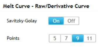
Viewing Graphical Displays of the Results 10
Configure and apply analysis templates
Agilent Aria Real-Time PCR Program 194
• At the top of the Analysis Term Settings dialog box, select Analysis
Criteria.
• Under the Background Based Threshold heading, in the first field
next to Cycle Range, type the cycle number that will be the first
cycle in the range, or click the +/- buttons to adjust the value in the
field to the desired cycle number.
• In the second field, type the cycle number that will be the last cycle
in the range, or click the +/- buttons to adjust the value in the field
to the desired cycle number.
• In the Sigma Multiplier field, type the desired value for the sigma
multiplier, or click the +/- buttons to adjust the value in the field to
the desired cycle number.
• Next to Smoothing, select On to turn on curve smoothing for the
amplification plots, or select Off to turn off curve smoothing.
• Click Apply to save changes.
2 (Optional) Set the Savitzky- Golay smoothing options for melt curves as
desired.
• At the top of the Analysis Term Settings dialog box, select Analysis
Criteria.
• Under Melt Curve - Raw/Derivative Curve, next to Savitzky- Golay,
select On to turn on smoothing for the melt curves, or select Off to
turn off smoothing.
• If you selected On, next to Points, select the number of data points
on each melt curve that you want the algorithm to use in the
smoothing calculations. A higher number of points leads to a
smoother (i.e., more manipulated) curve.
• Click Apply to save changes.
3 (Optional) Designate how data from replicate wells are treated during
analysis.
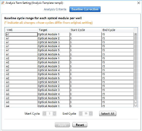
10 Viewing Graphical Displays of the Results
Configure and apply analysis templates
195 Agilent Aria Real-Time PCR Program
• At the top of the Analysis Term Settings dialog box, select Analysis
Criteria.
• Under General Settings, select Treat Individually to analyze each
well separately, or select Treat Collectively to average the data at
each cycle.
• Click Apply to save changes.
4 (Optional) Set the cycle range used for baseline correction.
Newly created analysis templates have the baseline cycle range set to
cycles 3–15. To obtain the optimal baseline value, you may need to
adjust the baseline cycle range in individual experiments. See “Adjust
the baseline correction settings” on page 199.
• Under Amplification Plots, set Baseline Correction to On. This
enables viewing and editing of the baseline correction cycle range for
the template.
• At the top of the Analysis Term Settings dialog box, select Baseline
Correction.
The dialog box displays the settings for the baseline cycle range.
Viewing Graphical Displays of the Results 10
Configure and apply analysis templates
Agilent Aria Real-Time PCR Program 196
• Select the plots (a plot is one target in one well) that you want to
adjust by clicking the appropriate row in the table. Press Ctrl while
clicking to select more than one plot. Click Select All to select all
plots in the table.
• In the Start Cycle field at the bottom of the dialog box, type the
cycle number that will be the first cycle in the baseline cycle range,
or click the +/- buttons to adjust the value in the field to the desired
cycle number.
• In the End Cycle field, type the cycle number that will be the last
cycle in the baseline cycle range, or click the +/- buttons to adjust
the value in the field to the desired cycle number.
• Click Apply to save changes.
5 When finished configuring the analysis template, click the red X in the
top right corner to close the Analysis Term Settings dialog box.

10 Viewing Graphical Displays of the Results
View the Amplification Plots
197 Agilent Aria Real-Time PCR Program
View the Amplification Plots
The Amplification Plots graph on the Graphical Displays screen shows a
plot of fluorescence (Y-axis) versus cycles (X-axis) for each target in each
well (or in each set of replicate wells) at a single data collection point.
The panel on the right side of the screen has tools for adjusting some of
the analysis parameters for the amplification plots.
To view the Amplification Plots: Click Graphical Displays in the
Experiment Area panel on the left side of the screen. If the Amplification
Plots graph is not already displayed, click the Amplification Plots icon at
the bottom of the screen.
View data for a single data point
Each curve on the amplification plots is the plot for a single target in a
single well or replicate set. Each data point that makes up the curve is a
fluorescence value (plotted on the Y- axis) measured at a particular cycle
number (plotted on the X- axis). The program connects these data points
to draw the curves displayed on the graph.
To view a summary of the data for a single data point on a plot:
1 Select the Amplification Plots graph on the Graphical Displays screen.
2 Hover your cursor over an individual plot on the graph.
A tooltip opens displaying the following information:
• Well ID and/or replicate number of the plot
• Target/dye
• Well type
• Fluorescence data type for the plot followed by the X and Y
coordinates for the data point where your cursor is located
• (If replicates are being treated individually) Baseline range (starting
cycle number, ending cycle number) used to calculate
baseline- corrected fluorescence values for that plot
Viewing Graphical Displays of the Results 10
View the Amplification Plots
Agilent Aria Real-Time PCR Program 198
Select a fluorescence data type
For the Y- axis of the amplification plots, you can select to use
fluorescence values that have been baseline- corrected and/or normalized
to a reference dye (if included).
To select the type of fluorescence data displayed in the amplification
plots:
1 Select the Amplification Plots graph on the Graphical Displays screen.
2 In the right panel, select one of the options next to Fluorescence Term.
The possible options are:
R - raw fluorescence
ΔR - baseline- corrected raw fluorescence
Rn - normalized fluorescence (normalized to the reference dye)
ΔRn - baseline- corrected and normalized fluorescence
If the thermal profile for your experiment included multiple data
collection points during amplification, see “Select which data collection
points to analyze” on page 181 for instructions on specifying which data
collection point to use for generating the amplification plots.
Specify the use of smoothing
You can select to apply a curve- smoothing algorithm to the amplification
plots. Smoothing alters the shapes of the amplification plots by decreasing
the effects of signal noise. The algorithm is based on a moving average
calculation with 5 averaging points.
The smoothing option is turned on by default.
To turn smoothing on or off:
1 Select the Amplification Plots graph on the Graphical Displays screen.
2 In the right panel, next to Smoothing, select On to turn on smoothing,
or select Off to turn off smoothing.

10 Viewing Graphical Displays of the Results
View the Amplification Plots
199 Agilent Aria Real-Time PCR Program
Adjust the graph properties
You can adjust certain properties of the Amplification Plots graph (e.g.,
the scales of the axes, the graph title, and the background color) through
the short- cut menu and the Graph Properties dialog box. See “Customize
graph properties” on page 240 for more information.
Adjust the baseline correction settings
By default, the program automatically determines which cycles to use to
calculate the baseline in order to produce baseline- corrected fluorescence
(ΔR) data for each well/target combination. For each target in each well,
the raw fluorescence data over a specific range of cycles are fit to a line
using a linear least mean squares algorithm to produce a baseline. The
value of the baseline function is calculated for every cycle and subtracted
from the raw fluorescence to produce baseline- corrected fluorescence
(ΔR).
You can view and adjust these software- determined cycle ranges (known
as adaptive values) from the Baseline Correction dialog box. You can
adjust the cycle range for individual plots, or set all plots to the same
cycle range.
To open the Baseline Correction dialog box:
1 Select the Amplification Plots graph on the Graphical Displays screen.
2 In the right panel, click the downward arrowhead above the result table
to display the advanced analysis parameter settings.
3 Next to Baseline Correction, click Adjust. (An asterisk on the Adjust
button indicates that the baseline settings have already been manually
adjusted.)
The Baseline Correction dialog box opens.
NOTE
If the Cq value for a target is within the baseline cycle range, the Aria software
calls the target as “no Cq.” In such cases, adjust the baseline cycle range for that
target to make sure that the Cq is not within the baseline cycle range.

Viewing Graphical Displays of the Results 10
View the Amplification Plots
Agilent Aria Real-Time PCR Program 200
To adjust the baseline cycle range:
1 Open the Baseline Correction dialog box.
2 Select the plots (a plot is one target in one well) that you want to
adjust by clicking the appropriate row in the table. Press Ctrl while
clicking to select more than one plot. Click Select All to select all plots
in the table.
3 In the Start Cycle field at the bottom of the dialog box, type the cycle
number that will be the first cycle in the baseline cycle range, or click
the +/- buttons to adjust the value in the field to the desired cycle
number.

10 Viewing Graphical Displays of the Results
View the Amplification Plots
201 Agilent Aria Real-Time PCR Program
4 In the End Cycle field, type the cycle number that will be the last cycle
in the baseline cycle range, or click the +/- buttons to adjust the value
in the field to the desired cycle number.
5 Click Apply to apply this baseline cycle range to the selected plots.
The program updates the table to show the new cycle range and adds
an asterisk (*) to the Well column to indicate that the cycle range for
that plot differs from the adaptive values.
To set the baseline cycle range back to adaptive values:
1 Open the Baseline Correction dialog box.
2 Select the plots (a plot is one target in one well) that you want to reset
to the adaptive values by clicking the appropriate line in the table.
Press Ctrl while clicking to select more than one plot. Click Select All
to select all plots in the table.
3 Click Reset.
The program updates the cycle ranges listed in the table back to the
adaptive values.
Adjust the crosstalk correction settings
Crosstalk occurs when emission from one dye is detected by two different
optical modules (the target optical module and the spillover optical
module). A dye is at risk for crosstalk when its emission wavelength
overlaps that of another dye that is assigned to a different optical module.
The Aria program includes crosstalk correction settings, which can help
compensate for crosstalk.
You can adjust the crosstalk correction settings for an individual
experiment from the Amplification Plots using the instructions provided
here. Alternatively, you can change the default crosstalk correction settings
for all new experiments going forward from the Supported Optical
NOTE
The factory settings for crosstalk correction have been optimized to eliminate
potential crosstalk for dyes that are part of the default optical configuration.
Agilent does not recommend changing the crosstalk correction settings unless
you are using a new custom dye and the emission wavelength of that dye could be
detected by more than one optical module in the instrument.

Viewing Graphical Displays of the Results 10
View the Amplification Plots
Agilent Aria Real-Time PCR Program 202
Configuration dialog box. The factory settings for crosstalk correction are
the default settings, unless the default settings are changed in the
Supported Optical Configuration dialog box. See “Change the default
crosstalk correction settings” on page 25 for instructions.
If you suspect that your custom dye may be detected by more than one
optical module, perform the following set of steps to eliminate crosstalk:
1 Run an experiment in which the custom dye is the only dye used in the
reactions. In the Plate Setup of the experiment, assign a target to the
spillover optical module as well as the target optical module for the
dye.
For example, if you are using the custom dye TET, then CY3 is the
target optical module and FAM is the spillover optical module. In the
Plate Setup, mark CY3 and FAM, as shown in the image below.
2 After running the experiment, view the results in the Amplification
Plots graph to determine if there is an increase in fluorescence
detected by the spillover optical module.
In the example Amplification Plots graph below, only the plots for the
spillover optical module (FAM) are displayed. A low level of
fluorescence from the TET dye is being detected by the FAM optical
module.

10 Viewing Graphical Displays of the Results
View the Amplification Plots
203 Agilent Aria Real-Time PCR Program
3 Adjust the crosstalk correction setting for the spillover optical module
until that optical module no longer detects an increase in fluorescence
(i.e., the amplification plot for the optical module is as close to flat as
possible in the graph). See instructions in “To adjust the crosstalk
correction settings:” on page 204 for details on how to perform this
step.
In the example Amplification Plots graph below, the crosstalk correction
setting for CY3 in the FAM optical module has been adjusted and the
plots are now nearly flat.

Viewing Graphical Displays of the Results 10
View the Amplification Plots
Agilent Aria Real-Time PCR Program 204
4 For all experiments that include this dye, make sure that the crosstalk
correction setting for the spillover optical module is set to the value
determined in Step 3 above. To change the default crosstalk correction
settings for future experiments, see “Change the default crosstalk
correction settings” on page 25.
To adjust the crosstalk correction settings:
1 Select the Amplification Plots graph on the Graphical Displays screen.
2 In the right panel, click the downward arrowhead above the result table
to display the advanced analysis parameter settings.
3 Next to Crosstalk Correction, click Adjust.
The Crosstalk Correction dialog box opens. The dialog box only displays
the settings for the optical modules used in the experiment. For each
optical module that is displayed, the current crosstalk correction setting
for each dye is listed.
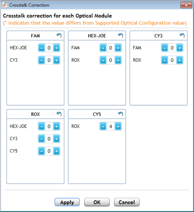
10 Viewing Graphical Displays of the Results
View the Amplification Plots
205 Agilent Aria Real-Time PCR Program
4 In the dialog box, locate the box for the optical module that is reporting
crosstalk fluorescence (i.e., the spillover optical module). The dyes that
have the potential to crosstalk with that optical module are listed in
that box (e.g., the ROX dye in the CY5 optical module).

Viewing Graphical Displays of the Results 10
View the Amplification Plots
Agilent Aria Real-Time PCR Program 206
5 Change the crosstalk correction setting for the dye by adjusting the
value in the field.
The values in these fields are percentages of the total raw fluorescence.
They will be subtracted from the raw fluorescence signal for the
spillover optical module when that dye is used as a target.
Crosstalk correction values that differ from the default values specified
in the Supported Optical Configuration dialog box are noted with an
asterisk (*). To reset a value back to its default, click the reset icon.
6 Click Apply to apply or changes, or click OK to apply your changes and
close the dialog box.
Select the scale (linear or log) of the Y-axis
By default, the fluorescence values on the Y- axis of the amplification plots
are in linear scale. You can quickly toggle between linear scale and log
scale from the Graphical Displays screen.
To select the scale of the Y- axis:
1 Select the Amplification Plots graph on the Graphical Displays screen.
2 In the right panel, click the downward arrowhead above the result table
to display the advanced analysis parameter settings.
3 Next to Graph Type, select Linear to plot the fluorescence values on a
linear scale, or select Log to plot the fluorescence values on a log scale.
The program adjust the amplification plots according to your selection.
10 Viewing Graphical Displays of the Results
View the Amplification Plots
207 Agilent Aria Real-Time PCR Program
Manually adjust threshold fluorescence values
The threshold fluorescence value for a target determines the target's Cq
value. The Cq is the cycle number at which the fluorescence level passes
the threshold. You can manually adjust the threshold fluorescence values
while viewing the amplification plots.
To adjust the threshold fluorescence value for a target by typing the
desired value:
1 Select the Amplification Plots graph on the Graphical Displays screen.
2 In the right panel, click the downward arrowhead above the result table
to display the advanced analysis parameter settings.
3 Under Threshold Fluorescence, type a new value into the field next to
the desired target, or click on the +/- buttons to adjust the value. If the
lock icon is in the locked position for the target, click on it to unlock
before the adjusting threshold. See “Lock or unlock the threshold
fluorescence values” on page 210 for more information.
The position of the corresponding horizontal line on the amplification
plots adjusts to the new threshold fluorescence value.
To adjust the threshold fluorescence value for a target by dragging the
threshold line on the Amplification Plots graph:
1 Select the Amplification Plots graph on the Graphical Displays screen.
The threshold fluorescence level for each target is displayed on the
graph as a horizontal line with a triangle marker along the Y- axis.
2 In the right panel, click the downward arrowhead above the result table
to display the advanced analysis parameter settings.
3 Under Threshold Fluorescence, locate the target that you want to
adjust. If the lock icon next to the target is in the locked position, click
on it to unlock it.
4 On the graph, hover your cursor over the triangle marker for the
threshold line that you want to adjust.
The cursor becomes a vertical, double- side arrow, and a tooltip box
opens displaying the name of the target and its current threshold
fluorescence value.

Viewing Graphical Displays of the Results 10
View the Amplification Plots
Agilent Aria Real-Time PCR Program 208
5 Click and drag the triangle marker to the desired position on the
Y- axis.
The program sets the threshold fluorescence value for that target its
new Y- axis value. The program also updates the value listed for that
target in the right panel.
To reset the threshold fluorescence value for a target back to the default
value calculated by the program:
1 Select the Amplification Plots graph on the Graphical Displays screen.
2 In the right panel, click the downward arrowhead above the result table
to display the advanced analysis parameter settings.
3 Under Threshold Fluorescence, click the Recalculate icon next to
the desired target.
The program resets the threshold fluorescence value in the field back to
the default value and adjusts the position of the corresponding
horizontal line on the Amplification Plots graph.

10 Viewing Graphical Displays of the Results
View the Amplification Plots
209 Agilent Aria Real-Time PCR Program
Adjust threshold fluorescence values by altering the algorithm settings
The default threshold fluorescence values calculated by the program are
background based thresholds. Background based thresholds are based on
the level of fluorescence noise in the background. The program calculates
the background noise from the levels of fluorescence present in the
selected wells (the wells included in the analysis) during the early cycles
of PCR before product begins to accumulate and the fluorescence levels
rise. By default, the cycles that the application uses for calculating the
background noise are cycles 5 through 9.
To calculate the threshold fluorescence values, the program then
multiplies the standard deviation (sigma) of the raw fluorescence in the
background cycles by a mathematical constant known as a sigma
multiplier. The default sigma multiplier is 10.
You can adjust the cycles used for calculating background noise and the
sigma multiplier used in the algorithm from the Graphical Displays screen.
Adjusting these settings results in a change to the threshold fluorescence
values.
To change the range of cycles used for determining background noise:
1 Select the Amplification Plots graph on the Graphical Displays screen.
2 In the right panel, click the downward arrowhead above the result table
to display the advanced analysis parameter settings.
The current cycle range is displayed in the Cycle Range fields under
Background Based Threshold.
3 In the first field next to Cycle Range, type the cycle number that will
be the first cycle in the range, or click the +/- buttons to adjust the
value in the field to the desired cycle number.
The program automatically recalculates the background noise and
adjusts the threshold fluorescence values for all targets that have not
been locked.

Viewing Graphical Displays of the Results 10
View the Amplification Plots
Agilent Aria Real-Time PCR Program 210
4 In the second field, type the cycle number that will be the last cycle in
the range, or click the +/- buttons to adjust the value in the field to the
desired cycle number.
The program automatically recalculates the background noise and
adjusts the threshold fluorescence values for all targets that have not
been locked.
To change the value of the sigma multiplier:
1 Select the Amplification Plots graph on the Graphical Displays screen.
2 In the right panel, click the downward arrowhead above the result table
to display the advanced analysis parameter settings.
3 In the Sigma Multiplier field under Background Based Threshold, type
the desired value for the sigma multiplier, or click the +/- buttons to
adjust the value in the field to the desired cycle number.
The program automatically recalculates the background noise and
adjusts the threshold fluorescence values for all targets.
Lock or unlock the threshold fluorescence values
You can lock the threshold fluorescence value for a given target. When
locked, the threshold fluorescence value is fixed and the functions related
to manually adjusting the threshold for that target are disabled.
Additionally, if you make changes to the dataset or adjust any of the
algorithm settings, the program does not recalculate the threshold
fluorescence for that target.
To lock the threshold fluorescence value for a particular target:
1 Select the Amplification Plots graph on the Graphical Displays screen.
2 In the right panel, click the downward arrowhead above the result table
to display the advanced analysis parameter settings.
3 Under the Threshold Fluorescence, click the lock icon next to the
target name.
The image of the lock icon changes from unlocked ( ) to locked ( ).
NOTE
To set an accurate threshold, you need to set the cycle range to be in the flat
baseline range for all plots.

10 Viewing Graphical Displays of the Results
View the Amplification Plots
211 Agilent Aria Real-Time PCR Program
To unlock the threshold fluorescence value for a particular target:
1 Select the Amplification Plots graph on the Graphical Displays screen.
2 In the right panel, click the downward arrowhead above the result table
to display the advanced analysis parameter settings.
3 Under the Threshold Fluorescence, click the lock icon next to the
target name.
The image of the lock icon changes from locked ( ) to unlocked ( ).
NOTE
The settings for the threshold fluorescence values and baseline cycle ranges on the
Amplification Plots graph directly impact Cq value calls. Prior to finalizing an analysis of
experimental results, verify that these settings align with the analysis requirements for
your assay.

Viewing Graphical Displays of the Results 10
View the Melt Curve - Raw/Derivative Curve
Agilent Aria Real-Time PCR Program 212
View the Melt Curve - Raw/Derivative Curve
For experiments that include a melt segment in the thermal profile, the
Melt Curve - Raw/Derivative Curve graph on the Graphical Displays screen
displays the fluorescence data collected during the melt segment (Y- axis)
as a function of temperature (X- axis). The panel on the right side of the
screen has tools for adjusting some of the analysis parameters for the melt
curves.
To view the Melt Curve - Raw/Derivative Curve: Click Graphical
Displays in the Experiment Area panel on the left side of the screen. If
the Melt Curve - Raw/Derivative Curve graph is not already displayed,
click the icon for this graph at the bottom of the screen.
About raw/derivative curves
When using SYBR Green or EvaGreen dye for detection, the raw/derivative
curves are used to verify that the predominant PCR products are
amplicons of the intended target. The graph plots fluorescence or the first
derivative of the fluorescence versus temperature. The temperatures
plotted on the graph are typically from a melt segment ramp that included
a data collection point.
Plotting results based on the first derivative multiplied by - 1 [fluorescence
term -R´(T) or - Rn´(T)] allows you to view the amplification products as
peaks on the graph, with each peak centered on the melting temperature
(Tm) for that product. Products with a Tm of 80°C or higher correspond
to the larger PCR products, and can usually be assigned as specific DNA
product. Products displaying melting temperatures of <75°C correspond to
non- specific DNA products, such as primer dimers. It is important to note,
however, that these populations are not necessarily homogeneous, and may
contain multiple PCR product species.
10 Viewing Graphical Displays of the Results
View the Melt Curve - Raw/Derivative Curve
213 Agilent Aria Real-Time PCR Program
View data for a single data point
Each curve on the graph is the plot for a single target in a single well or
replicate set. Each data point that makes up the curve is a fluorescence
value (plotted on the Y- axis) measured at a particular temperature
(plotted on the X- axis). The program connects these data points to draw
the raw/derivative curves displayed on the graph.
To view a summary of the data for a single data point on a plot:
1 Select the Melt Curve - Raw/Derivative Curve graph on the Graphical
Displays screen.
2 Hover your cursor over an individual plot on the graph.
A tooltip opens displaying the following information:
• The well ID or replicate number for the plot and the target name
• The fluorescence data type for the plot followed by the X and Y
coordinates for the data point where your cursor is located
• The Tm of each product identified by the algorithm
Select a fluorescence data type
For the Y- axis of the raw/derivative curves, you can select to use raw or
normalized fluorescence values or the first derivative of those values
multiplied by - 1. Typically, the graphs are plotted using first derivative
values multiplied by - 1.
To select the type of fluorescence data displayed in the Raw/Derivative
Curve:
1 Select the Melt Curve - Raw/Derivative Curve graph on the Graphical
Displays screen.
2 In the right panel, select one of the options next to Fluorescence Term.
The possible options are:
R- Raw fluorescence
Rn-Normalized fluorescence (normalized to reference dye)
-R´(T)- First derivative of the raw fluorescence multiplied by - 1
-Rn´(T)- First derivative of the normalized fluorescence multiplied by - 1
Viewing Graphical Displays of the Results 10
View the Melt Curve - Raw/Derivative Curve
Agilent Aria Real-Time PCR Program 214
See “Select which data collection points to analyze” on page 181 for
information on specifying which data collection point to use for generating
the raw/derivative curves.
Adjust the graph properties
You can adjust certain properties of the Melt Curve - Raw/Derivative
Curve graph (e.g., the scales of the axes, the graph title, and the back
ground color) through the short- cut menu and the Graph Properties dialog
box. See “Customize graph properties” on page 240 for more information.
Specify the use of smoothing
You can select to apply a Savitzky- Golay curve- smoothing algorithm to the
raw/derivative curves [for a reference, see Savitzky and Golay, Analytical
Chemistry, 1964; 36(8):1627- 1639]. Smoothing alters the shapes of the
curves by decreasing the effects of signal noise. The smoothing option is
turned on by default.
To turn smoothing on or off:
1 Select the Melt Curve - Raw/Derivative Curve graph on the Graphical
Displays screen.
2 In the right panel, click the downward arrowhead above the result table
to display the advanced analysis parameter settings.
3 Next to Savitzky- Golay, select On to turn on smoothing, or select Off
to turn off smoothing.
4 If you selected On, next to Number of Points, select the number of
data points on each melt curve that you want the algorithm to use in
the smoothing calculations.
The options are 5, 7, 9, and 11. A higher number of points leads to a
smoother (i.e., more manipulated) curve.
Normalize the fluorescence values
To facilitate comparison among the curves on the graph, you can select to
normalize the fluorescence values on the Y- axis. Normalization rescales
the Y- axis value of each data point in each curve such that the minimum
10 Viewing Graphical Displays of the Results
View the Melt Curve - Raw/Derivative Curve
215 Agilent Aria Real-Time PCR Program
fluorescence value for each plot is set to 0 and the maximum fluorescence
value is set to 1. The normalization option is turned off by default.
To turn normalization on or off:
1 Select the Melt Curve - Raw/Derivative Curve graph on the Graphical
Displays screen.
2 In the right panel, click the downward arrowhead above the result table
to display the advanced analysis parameter settings.
3 Next to Normalization, select On to turn on normalization, or select
Off to turn off normalization.
Adjust the range of the X-axis
You can quickly modify the range of temperatures displayed on the X- axis.
To adjust the range of the X- axis:
1 Select the Melt Curve - Raw/Derivative Curve graph on the Graphical
Displays screen.
2 In the right panel, click the downward arrowhead above the result table
to display the advanced analysis parameter settings.
3 In the fields below Temperature Range, type in the desired lower
temperature and upper temperature for the X- axis range, or click the
+/- buttons to adjust the temperatures in the fields to the desired
values.
The program adjusts the range of the X- axis accordingly.

Viewing Graphical Displays of the Results 10
View the Melt Curve - Raw/Derivative Curve
Agilent Aria Real-Time PCR Program 216
Adjust product melting temperature settings
Some of the settings that the program uses to identify amplification
products and calculate melting temperatures are adjustable. You can
change the maximum number of amplification products for which the
program reports a melting temperature. When basing plots on the negative
derivative of fluorescence, you can set a minimum height that a product
peak must reach in order for the program to consider it an amplification
product.
To change the maximum number of amplification products for a which a
melting temperature is reported:
1 Select the Melt Curve - Raw/Derivative Curve graph on the Graphical
Displays screen.
2 In the right panel, click the downward arrowhead above the result table
to display the advanced analysis parameter settings.
3 In the Max Number field, below the Product Melting Temperature
heading, type in the desired maximum number of products, or click the
+/- buttons to adjust the number of products in the field to the desired
value. The default value is 4. The highest value allowed is 6.
To set a minimum peak height for an amplification product:
1 Select the Melt Curve - Raw/Derivative Curve graph on the Graphical
Displays screen.
2 In the right panel, click the downward arrowhead above the result table
to display the advanced analysis parameter settings.
3 Next to Min Peak Height, select On to turn on the minimum peak
height option.
A new field appears for entering the minimum peak height, and a
horizontal line appears on the graph marking the minimum height.
10 Viewing Graphical Displays of the Results
View the Melt Curve - Raw/Derivative Curve
217 Agilent Aria Real-Time PCR Program
4 In the field, type the desired minimum peak height, or click the +/-
buttons to adjust the value in the field. (Clicking the Reset icon sets the
Minimum Peak Height value to the lowest peak among the set of highest
peaks across all selected wells.)
The height of the horizontal line on the graph adjusts accordingly, and
the program only counts a peak as an amplification product if the peak
crosses that horizontal line.

Viewing Graphical Displays of the Results 10
View the Melt Curve - Difference Plots
Agilent Aria Real-Time PCR Program 218
View the Melt Curve - Difference Plots
The Melt Curve - Difference Plots graph on the Graphical Displays screen
is typically used for analysis of Allele Discrimination experiments that use
a DNA binding dye and a high resolution melt (HRM) segment to
distinguish between alleles. The graph displays the difference in
fluorescence between two plots during a melt ramp (Y- axis) as a function
of temperature (X- axis). The panel on the right side of the screen has
tools for adjusting some of the analysis parameters for the melt curves.
The Melt Curve - Difference Plots graph is only available for experiments
with:
• A high resolution melt (HRM) segment in the thermal profile
• An associated HRM calibration plate (HCP); see “Assign an HRM
calibration plate” on page 183.
To view the Melt Curve - Difference Plots: Click Graphical Displays in
the Experiment Area panel on the left side of the screen. If the Melt
Curve - Difference Plots graph is not already displayed, click the icon for
this graph at the bottom of the screen.
If the Difference Plots icon has a warning symbol next to it, then you
cannot open the Difference Plots until you assign an HRM calibration plate
(HCP) to the experiment. See “Assign an HRM calibration plate” on
page 183 for instructions.
About difference plots
Difference plots are a useful way of viewing the results of an Allele
Discrimination experiment that uses high resolution melt (HRM) analysis
for SNP (single nucleotide polymorphism) genotyping. The values plotted
on the Y- axis are the difference in fluorescence between a target in one
well (or replicate set) and a control target from a designated well/replicate
set. Because the plots display the difference in fluorescence, you can
detect even slight differences between two plots. Consequently, this graph
allows you to use HRM analysis to distinguish between product
populations that differ in sequence by as little as a single nucleotide.
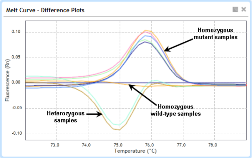
10 Viewing Graphical Displays of the Results
View the Melt Curve - Difference Plots
219 Agilent Aria Real-Time PCR Program
The equation for determining the Y- axis value at each temperature is:
Diff(T) = R(T) – compR(T)
where R(T) is the fluorescence value for the target at temperature T,
and compR(T) is the value for the control target at temperature T.
Note that the fluorescence value can be any fluorescence term [R, Rn,
–R´(T) or –Rn´(T)].
The figure below displays a difference plot for a class 4 SNP (A>T). Note
the distinctly different plot shape for each genotype group.
To use HRM analysis for SNP genotyping, your experiment needs to
include positive control samples for each base pair possibility (homozygous
as well as heterozygous positive control samples). Then, when viewing the
difference plots, designate the target in one of the homozygous positive
control samples as the control target. You can then compare samples of
unknown genotype to the samples of known genotype to visually
determine the correct genotype group for the target in the unknown
sample.
Viewing Graphical Displays of the Results 10
View the Melt Curve - Difference Plots
Agilent Aria Real-Time PCR Program 220
Select a fluorescence data type
For the Y- axis of the difference plots, you can select to use raw or
normalized fluorescence values.
To select the type of fluorescence data displayed in the Difference Plots:
1 Select the Melt Curve - Difference Plots graph on the Graphical
Displays screen.
2 In the right panel, select one of the options next to Fluorescence Term.
The possible options are:
R- Raw fluorescence
Rn-Normalized fluorescence (normalized to reference dye)
Assign the control target
The values plotted on the Y- axis are the difference in fluorescence values
between a target in a particular well (or replicate set) and a specified
control target. You can designate the control sample and target using the
using the tools in the panel on the right side of the screen. Typically, a
target from a homozygous positive control sample is selected as the
control.
To assign the control target:
1 Select the Melt Curve - Difference Plots graph on the Graphical
Displays screen.
2 In the right panel, click the downward arrowhead above the result table
to display the Control Target settings.
3 Under Control Target, use the drop- down lists to specify the well or
replicate set that contains the control sample and the target in that
well/replicate set that is detecting the control target.
a In the Well Type drop- down list, select the well type in which the
control target was amplified. Typically, one of the homozygous
control wells is selected (Homo Allele A or Homo Allele B).
b In the Replicate or Well Id drop- down list, select the specific well or
replicate set in which the control target was amplified.
c In the Target drop- down list, select the dye or target name for the
control target.

10 Viewing Graphical Displays of the Results
View the Melt Curve - Difference Plots
221 Agilent Aria Real-Time PCR Program
View data for a single data point
Each curve on the graph is the plot for a single target in a single well or
replicate set. Each data point that makes up the curve is a fluorescence
value for that target/well measured at a particular temperature (plotted on
the X- axis). The program connects these data points to draw the
raw/derivative curves displayed on the graph.
To view a summary of the data for a single data point on a plot:
1 Select the Melt Curve - Difference Plots graph on the Graphical
Displays screen.
2 Hover your cursor over an individual plot on the graph.
A tooltip opens displaying the following information:
• The well ID or replicate number for the plot and the dye/target name
• The fluorescence data type for the plot followed by the X and Y
coordinates for the data point where your cursor is located
• The Tm of each product identified by the algorithm
Manually assign Unknowns to a genotype call
Typically, you can visually examine the difference plots to determine the
genotype of the samples in the Unknown wells. Once you have made your
determinations, you can assign a genotype call to the Unknown
wells/replicate sets in the program.
Add the Call column to the Results table
Before assigning genotype calls, you may want to add the Call column to
the Results Table so you can easily see the call assignments. The calls you
apply appear in this column.
To add the Call column:
1 Click the Column Option icon above the table to open the Column
Options dialog box.
2 In the dialog box, mark Call.
3 Click OK.
The dialog box closes and the Call column appears in the Results Table.

Viewing Graphical Displays of the Results 10
View the Melt Curve - Difference Plots
Agilent Aria Real-Time PCR Program 222
Apply calls
To apply a genotype call to a single Unknown well or replicate set:
1 Select the Melt Curve - Difference Plots graph on the Graphical
Displays screen.
2 In the Results Table, locate the row for the well or replicate set of
interest, and right- click directly on that row.
3 In the pop- up menu that opens, click Apply Call to Current Item, then
click the genotype that you want to assign (Homozygous A, Homozygous
B, or Heterozygous).
If the Results Table is displaying the Call column, the call you applied
appears in that column.
To apply a genotype call to multiple Unknown wells or replicates sets:
1 Select the Melt Curve - Difference Plots graph on the Graphical
Displays screen.
2 In the Results Table, add the Check column (if not already added).
a Click the Column Option icon above the table to open the
Column Options dialog box.
b Mark Check and click OK.
3 In the Results Table, locate the wells or replicate sets that you want to
assign to the same genotype call. For those wells or replicate sets, mark
the check box in the Check column.
4 Right- click on the Results Table or on the Difference Plots graph.
5 In the pop- up menu that opens, click Apply Call to All Checked Items,
then click the genotype that you want to assign (Homozygous A,
Homozygous B, or Heterozygous).
If the Results Table is displaying the Call column, then the call you
applied appears in that column.
Clear calls
You can remove calls that were manually applied to Unknown wells or
replicate sets.

10 Viewing Graphical Displays of the Results
View the Melt Curve - Difference Plots
223 Agilent Aria Real-Time PCR Program
To clear a call for a single Unknown well or replicate set:
1 Select the Melt Curve - Difference Plots graph on the Graphical
Displays screen.
2 In the Results Table, locate the row for the well or replicate set of
interest, and right- click directly on that row.
3 In the pop- up menu that opens, click Apply Call to Current Item >
Clear Call.
If the Results Table is displaying the Call column, the call no longer
appears in that column.
To clear a call from multiple Unknown wells or replicate sets:
1 Select the Melt Curve - Difference Plots graph on the Graphical
Displays screen.
2 In the Results Table, add the Check column (if not already added).
a Click the Column Option icon above the table to open the
Column Options dialog box.
b Mark Check and click OK.
c In the Results Table, locate the wells or replicate sets for which you
want to clear the manually applied genotype call. For those wells or
replicate sets, mark the check box in the Check column.
d Right- click on the Results Table or on the Difference Plots graph.
e In the pop- up menu that opens, click Clear All Checked Items.
If the Results Table is displaying the Call column, the calls no longer
appears in that column.
Edit manual call settings
From the HRM Manual Calling dialog box, you can edit the name and
color that is used to for each genotype in the Difference Plots graph and
the result table.
1 Select the Melt Curve - Difference Plots graph on the Graphical
Displays screen.
2 Right- click on the Results Table or on the Difference Plots graph.
3 In the pop- up menu that opens, click Edit Manual Call Settings.
The HRM Manual Calling dialog box opens.
Viewing Graphical Displays of the Results 10
View the Melt Curve - Difference Plots
Agilent Aria Real-Time PCR Program 224
4 For the genotype that you want to assign to a different name, type the
desired name into the field.
5 For the genotype that you want to assign to a different color, expand
the drop- down list to view the color options.
6 Click directly on the color that you want to assign.
7 Click OK in the dialog box.
The dialog box closes and color coding in the difference plots is
updated.
Adjust the graph properties
You can adjust certain properties of the Melt Curve - Difference Plots
graph (e.g., the scales of the axes, the graph title, and the background
color) through the short- cut menu and the Graph Properties dialog box.
See “Customize graph properties” on page 240 for more information.

10 Viewing Graphical Displays of the Results
View the Standard Curve
225 Agilent Aria Real-Time PCR Program
View the Standard Curve
For Quantitative PCR experiments, Comparative Quantitation experiments,
and User Defined experiments that include a set of Standard wells, the
Graphical Displays screen includes a Standard Curve graph. This graph is
a plot of the Cq (Y- axis) versus the log of the initial template quantity in
the Standard wells (X- axis). Each plot is a target in a Standard well or
replicate set. The graph also plots the Cq values from the Unknown wells.
The program uses a least mean squares curve fitting algorithm to generate
the standard curves. The panel on the right side of the screen has tools
for adjusting some of the analysis parameters.
To view the Standard Curve: Click Graphical Displays in the Experiment
Area panel on the left side of the screen. If the Standard Curve graph is
not already displayed, click the Standard Curve icon at the bottom of the
screen.
View data for a single data point
Each curve on the graph is the plot for a single target in a single
Standard well or replicate set. The square- shaped markers denote the data
points from the Standard wells that make up the curve. Each of these
data points is a fluorescence value (typically log scale) plotted against the
initial template quantity as entered on the Plate Setup screen. The
program connects these data points to draw the curves displayed on the
graph. The triangle- shaped markers on the graph denote Cq values from
Unknown wells.
To view a summary of the data for a single data point from a Standard
well:
1 Select the Standard Curve graph on the Graphical Displays screen.
2 Hover your cursor over the square marker for the data point of interest.
A tooltip opens displaying the following information:
NOTE
Only the Standard wells that you selected in the Analysis Criteria screen are
included in the Standard Curve graph.
Viewing Graphical Displays of the Results 10
View the Standard Curve
Agilent Aria Real-Time PCR Program 226
• The well ID, replicate number, target name, and well type (or sample
name) for the plot
• The initial template quantity as entered on the Plate Setup screen
(i.e., the X- axis coordinate)
• The quantification cycle for the plot (i.e., the Y- axis coordinate)
To view a summary of the data for a single data point from an Unknown
well:
1 Select the Standard Curve graph on the Graphical Displays screen.
2 Hover your cursor over the triangle marker for the data point of
interest.
A tooltip opens displaying the following information:
• The well ID, replicate number, target name, and well type (or sample
name) for the plot
• The initial template quantity as calculated by the program (i.e., the
X- axis coordinate)
• The quantification cycle for the plot (i.e., the Y- axis coordinate)
Select a fluorescence data type
For the Y- axis of the amplification plots, you can use baseline- corrected
fluorescence values with or without normalization to a reference dye.
To select the type of fluorescence data displayed in the Standard Curve
graph:
1 Select the Standard Curve graph on the Graphical Displays screen.
2 In the right panel, select one of the options next to Fluorescence Term.
The possible options are:
ΔR - baseline- corrected raw fluorescence
ΔRn - baseline- corrected, normalized fluorescence
See “Select which data collection points to analyze” on page 181 for
information on specifying which data collection point to use for generating
the standard curve.
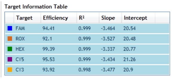
10 Viewing Graphical Displays of the Results
View the Standard Curve
227 Agilent Aria Real-Time PCR Program
View the R-squared values, slopes, and amplification efficiencies
The Target Information Table displays information about each target on
the Standard Curve graph. This information includes the amplification
efficiency (which is calculated from the slope), the R- squared (R
2
) value,
the slope of the standard curve plot, and the point where it intercepts the
Y- axis.
The R
2
value is an indicator of the quality of the fit of the standard curve
to the standard data points plotted. The value is always between 0 and 1,
and the closer the value is to 1, the better the fit of the line.
The slope of the curve is directly related to the average amplification
efficiency throughout the cycling reaction. The program uses the following
equation to calculate slope:
y = m*log(x) + b, where m is the slope of the line
PCR efficiency is the percentage of template molecules that are doubled
every cycle. The equation that relates the slope to amplification efficiency
is:
PCR efficiency = 10(- 1/slope) - 1
Based on this equation, a PCR reaction with 100% efficiency results in a
standard curve with a slope of - 3.322.
To view the Target Information Table:
1 Select the Standard Curve graph on the Graphical Displays screen.
The table is displayed in the panel on the right side of the screen.

Viewing Graphical Displays of the Results 10
View the Standard Curve
Agilent Aria Real-Time PCR Program 228
Adjust the graph properties
You can adjust certain properties of the Standard Curve graph (e.g., the
scales of the axes, the graph title, and the background color) through the
short- cut menu and the Graph Properties dialog box. See “Customize
graph properties” on page 240 for more information.
Manually adjust threshold fluorescence values
The threshold fluorescence value for a target determines the target's Cq
value. The Cq is the cycle number at which the fluorescence level passes
the threshold. You can manually adjust the threshold fluorescence values
while viewing the standard curves.
To adjust the threshold fluorescence value for a target by typing the
desired value:
1 Select the Amplification Plots graph on the Graphical Displays screen,
and unlock the threshold fluorescence values that you want to manually
adjust.
2 Select the Standard Curve graph.
3 In the right panel, click the downward arrowhead above the result table
to display the advanced analysis parameter settings.
4 Under Threshold Fluorescence, type a new value into the field next to
the desired target, or click on the +/- buttons to adjust the value.
The program adjusts the standard curves according to the new values.
To reset the threshold fluorescence value for a target back to the default
value calculated by the program:
1 Select the Standard Curve graph on the Graphical Displays screen.
2 In the right panel, click the downward arrowhead above the result table
to display the advanced analysis parameter settings.
3 Under Threshold Fluorescence, click the Recalculate icon next to
the desired target.
The program resets the threshold fluorescence value in the field back to
the default value and adjusts the standard curves accordingly.
10 Viewing Graphical Displays of the Results
View the Standard Curve
229 Agilent Aria Real-Time PCR Program
Display and adjust confidence intervals
You can select to display the confidence intervals for each plot on the
Standard Curve graph as hashed lines. These lines show the range of
initial quantity values at a particular Cq that cannot be statistically
distinguished from the fit line with more certainty than the specified
confidence level. The width of the confidence interval is an indicator of
the quality of the fit of the data to the standard curve.
The default confidence level is 99%. When you select to display the
confidence intervals, you can adjust the confidence level.
To display confidence intervals, the program must treat replicates
individually.
To display confidence intervals:
1 Select the Standard Curve graph on the Graphical Displays screen.
2 In the right panel, click the downward arrowhead above the result table
to display the advanced analysis parameter settings.
3 Under Threshold Fluorescence, mark Show confidence interval.
The program displays the hashed lines on the Standard Curve graph
indicating the confidence intervals.
If you had selected to treat replicates collectively, the program will
prompt you to treat them individually in order to display the intervals.
To adjust the confidence level:
1 Display the confidence intervals on the Standard Curve graph (see
instructions above).
2 Next to Level %, type the desired confidence level into the field, or
click on the +/- buttons to adjust the value in the field.
The program updates the positions of the confidence interval lines on
the graph to reflect the new confidence level.

Viewing Graphical Displays of the Results 10
View the Relative Quantity
Agilent Aria Real-Time PCR Program 230
View the Relative Quantity
For Comparative Quantitation experiments and User Defined experiments
that include a set of Calibrator wells, the Graphical Displays screen
includes a Relative Quantity chart. This chart is a bar graph that shows
the amount of target present in the experimental samples (the Unknown
wells) relative to the associated reference sample (the Calibrator wells)
after the program has normalized the quantities using data from the
normalizer target.
To view the Relative Quantity: Click Graphical Displays in the
Experiment Area panel on the left side of the screen. If the Relative
Quantity chart is not already displayed, click the Relative Quantity icon at
the bottom of the screen.
About relative quantities
Each bar on the graph is a target within a well or replicate set. The
expression level of the target- of- interest in the Calibrator wells is defined
1.0. In the Unknown wells, the expression levels of the target- of- interest
are reported on the Y- axis as a fold difference relative to the calibrator
benchmark.
How you set up the wells on the Plate Setup screen impacts how the
program compares samples in the Relative Quantity chart.
• If you designate a separate calibrator sample for each unique target, the
program only compares Unknown wells with that same target to those
Calibrator wells. This allows you to run multiple targets on the same
plate and analyze them independently.
• If you set up multiple Calibrator wells/replicate sets with the same
target name, the program will average the Cq values of those Calibrator
wells and calculate the relative quantities of that target in the Unknown
wells relative to the average.
10 Viewing Graphical Displays of the Results
View the Relative Quantity
231 Agilent Aria Real-Time PCR Program
Select a fluorescence data type
For the Y- axis of the Relative Quantity chart, you can use
baseline- corrected fluorescence values with or without normalization to a
reference dye.
To select the type of fluorescence data displayed in the Relative Quantity
chart:
1 Select the Relative Quantities chart on the Graphical Displays screen.
2 In the right panel, select one of the options next to Fluorescence Term.
The possible options are:
ΔR - baseline- corrected raw fluorescence
ΔRn - baseline- corrected, normalized fluorescence
Set the Y-axis scale for the Relative Quantity chart
By default, the program displays the Y- axis in linear scale. In this scale,
you can view the quantity of an target as a fold change in expression level
relative to the calibrator. This view is convenient for assessing increases in
expression levels of a target relative to the calibrator.
Alternatively, you can set the Y- axis to display the target quantities on a
base 2- logarithmic scale. This view is convenient for viewing target
expression levels that decrease or increase relative to the calibrator.
To display the relative quantities of the targets in the Unknown wells on a
base 2- logarithmic scale:
1 Select the Relative Quantity chart on the Graphical Displays screen.
2 In the right panel next to Chart Type, select Log2.
The program updates the Y- axis values on the chart.
To reset the chart to display relative quantities as a fold change relative to
the quantities in the Calibrator wells:
1 Select the Relative Quantity chart on the Graphical Displays screen.
2 In the right panel next to Chart Type, select Fold.
The program updates the Y- axis values on the chart.
Viewing Graphical Displays of the Results 10
View the Relative Quantity
Agilent Aria Real-Time PCR Program 232
Add error bars to the Relative Quantity chart
When you are treating replicate wells collectively, you can select to display
error bars on the relative quantities that reflect the deviation among the
replicates. The program calculates the error bars on the relative quantities
from the error bars on the Cqs, which it calculates from the deviation on
each fluorescence measurement at each cycle and estimates on the
imprecision of the normalizers.
To add error bars:
1 Select the Relative Quantity chart on the Graphical Displays screen.
2 Make sure that the program is set to treat replicates collectively. (See
“Choose a treatment for replicate wells” on page 182.)
3 In the right panel next to Error Bar, select On.
The program add error bars to the chart.
To remove error bars:
1 Select the Relative Quantity chart on the Graphical Displays screen.
2 In the right panel next to Error Bar, select Off.
The program removes the error bars from the chart.
Adjust the graph properties
You can adjust certain properties of the Relative Quantities chart (e.g., the
scales of the axes, the graph title, and the background color) through the
short- cut menu and the Graph Properties dialog box. See “Customize
graph properties” on page 240 for more information.
Select the algorithm method
The program provides multiple algorithm options for calculating the
relative quantities.
To select an algorithm for the relative quantity calculations:
1 Select the Relative Quantity chart on the Graphical Displays screen.
2 In the right panel, click the downward arrowhead above the result table
to display the advanced analysis parameter settings.
10 Viewing Graphical Displays of the Results
View the Relative Quantity
233 Agilent Aria Real-Time PCR Program
3 Next to Mode, select the method you want to use. The options are
described briefly below.
ΔΔCq (Livak) - The ΔΔCq method, also called the Livak method, relies
on two assumptions. The first assumption is that both the normalizer
and the target- of- interest have amplification efficiencies at or near
100% and that the efficiencies of the two targets do not differ by more
than 5%. The second assumption is that the amplification efficiency of a
target is consistent from one run to the next. Any run- to- run variance
is not included in the calculations. The ΔΔCq method is often referred
to as an approximation method and requires a validation step to
confirm that efficiencies of your normalizer and target- of- interest are
similar. This method is only available if the wells selected on the
Analysis Criteria screen include a normalizer target.
ΔCq - The ΔCq method is similar to the ΔΔCq method in that it relies
on the same mathematical assumptions about efficiencies and
consistency. Unlike the ΔΔCq method, however, the relative quantity in
the calibrator sample is not set to 1.0. This method is only available if
the wells selected on the Analysis Criteria screen do not include a
normalizer target.
Pfaffl - With the Pfaffl method, the program takes into account the
amplification efficiencies of the normalizer and target- of- interest when
calculating the relative quantities. This method is a good choice for
Comparative Quantitation experiments in which the normalizer and
target- of- interest differ in amplification efficiency. The Pfaffl method
does not, however, incorporate run- to- run variations in amplification
efficiency. For a reference, see: Pfaffl, M. W. (2001) Nucleic Acids Res.
29(9):e45. This method is only available if the wells selected on the
Analysis Criteria screen include a normalizer target.
Enter the amplification efficiencies for the targets
If you selected the Pfaffl algorithm method to calculate the relative
quantities, you need to enter the amplification efficiency of each target. If
you determined the efficiencies based on a standard curve that was run in
another experiment, you can enter the efficiencies manually. If the current
experiment includes a standard curve to determine the efficiencies, you
can specify to use the efficiencies derived from that data.
Viewing Graphical Displays of the Results 10
View the Relative Quantity
Agilent Aria Real-Time PCR Program 234
To enter the amplification efficiencies manually:
1 Select the Relative Quantity chart on the Graphical Displays screen.
2 In the right panel, click the downward arrowhead above the result table
to display the advanced analysis parameter settings.
3 Next to Mode, select Pfaffl to enable the fields in the Amplification
Efficiencies table.
4 In the Amplification Efficiencies table, enter the efficiency of each
target using either of the following approaches:
• In the Slope column, type the slope of the target, or click the +/-
buttons to adjust the value in the field. The program automatically
adjusts the value in the Efficiency (%) column by relating slope to
amplification efficiency.
• In the Efficiency (%) column, type the amplification efficiency of the
target, or click the +/- buttons to adjust the value in the field. The
program automatically adjusts the value in the Slope column by
relating amplification efficiency to slope.
To enter the amplification efficiencies from a standard curve included in
the experiment:
1 Select the Relative Quantity chart on the Graphical Displays screen.
2 In the right panel, click the downward arrowhead above the result table
to display the advanced analysis parameter settings.
3 Next to Mode, select Pfaffl to enable the fields in the Amplification
Efficiencies table.
4 Below the Amplification Efficiencies table, mark the check box labeled
Apply Std Curve Efficiencies to CQ Results.

10 Viewing Graphical Displays of the Results
View the Allele Determination graph
235 Agilent Aria Real-Time PCR Program
View the Allele Determination graph
For Allele Discrimination experiments and User Defined experiments that
include wells with allele designations, the Graphical Displays screen
includes an Allele Determination graph. This graph is useful for viewing
the genotype results in Allele Discrimination experiments that use two
differentially- labeled fluorescent probes to detect the two different alleles.
Each plotted point on the graph represents the coordinates of either the
fluorescence values or Cq values for the two targets. For example, the
X- axis may correspond to the Cq of the Allele A target while the Y- axis
corresponds to the Cq of the Allele B target and the plotted point (x,y)
corresponds to the coordinates describing the two Cq values determined
for a given well. The position of the data point on the graph indicates the
presence or absence of each allele.
To view the Allele Determination: Click Graphical Displays in the
Experiment Area panel on the left side of the screen. If the Allele
Determination graph is not already displayed, click the icon for this graph
at the bottom of the screen.
View data for a single data point
If you set up the experiment to amplify the two alleles within the same
well, then each data point on the Allele Determination graph represents a
single well or replicate set. If you set up the experiment to amplify the
two alleles in separate wells that contain the same sample, then each data
point represents a single sample.
To view a summary of the data for a single data point on a plot:
1 Select the Allele Determination graph on the Graphical Displays screen.
2 Hover your cursor over an individual data point on the graph.
A tooltip opens displaying the following information:
• The well ID or replicate number for the data point
• The fluorescence data type for the plot followed by the X and Y
coordinates for the data point
• The well name as specified on the Plate Setup screen
Viewing Graphical Displays of the Results 10
View the Allele Determination graph
Agilent Aria Real-Time PCR Program 236
• The genotype assigned by the program to that target in that
well/replicate
Select data type and fluorescence type to display
Each plotted point on the graph represents the coordinates of either the
fluorescence values or Cq values for the two targets. You can select which
type of data (fluorescence or Cq) you want displayed on the graph.
To select a data type and fluorescence type:
1 Select the Allele Determination graph on the Graphical Displays screen.
2 In the right panel, next to Display by, select Fluorescence to plot the
fluorescence values, or select Cq to plot the Cq values.
Based on your selection, the program displays the options for
fluorescence data type.
3 Select one of the fluorescence data type options.
• The possible options if you selected to display by Fluorescence:
R last - the final raw fluorescence reading as measured in the last
cycle
ΔR last - the final baseline- corrected fluorescence reading as
measured in the last cycle
Rn last - the final normalized fluorescence reading as measured in
the last cycle
ΔRn last - the final baseline- corrected, normalized fluorescence
reading as measured in the last cycle
R last / R first - the final fluorescence reading divided by the initial
fluorescence reading
• The possible options if you selected to display by Cq:
ΔR - Cq of the baseline- corrected raw fluorescence plot
ΔRn - Cq of the baseline- corrected and normalized fluorescence plot
See “Select which data collection points to analyze” on page 181 for
information on specifying which data collection point to use for generating
the amplification plots.
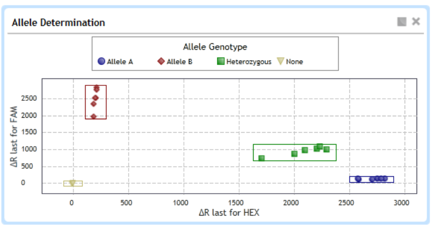
10 Viewing Graphical Displays of the Results
View the Allele Determination graph
237 Agilent Aria Real-Time PCR Program
Display genotype groups on the graph
You can include on the graph colored rectangles that group data points
with the same assigned genotype (allelic composition). You can allow the
program to automatically determine the positions of these rectangles, or
you can manually position them yourself.
To include colored rectangles that are automatically determined by the
program:
1 Select the Allele Determination graph on the Graphical Displays screen.
2 In the right panel, next to Genotype Calls, select Auto.
The program adds the rectangles to the graph, grouping data points
with the same genotype call.
To include colored rectangles and manually position them:
1 Select the Allele Determination graph on the Graphical Displays screen.
2 In the right panel, next to Genotype Calls, select Manual.
The program adds the rectangles to the graph, grouping data points
with the same genotype call.
Viewing Graphical Displays of the Results 10
View the Allele Determination graph
Agilent Aria Real-Time PCR Program 238
3 Move the border of the any of the rectangles to include or exclude data
points.
a Hover your cursor over the border that you want to reposition.
b Click and drag the border to a new position.
To specify which genotype groups have a rectangle displayed on the graph:
1 Select the Allele Determination graph on the Graphical Displays screen.
2 Right- click on the graph.
A short- cut menu opens. The menu includes a list of the possible
genotypes (Allele A, Allele B, Both, and None). The genotypes that are
already represented on the graph with a rectangle have a check mark
next to them.
3 Click on the genotypes in the short- cut menu to add or remove
rectangles as desired.
Each time you click a genotype, the short- cut menu closes and the
program updates the rectangles on the graph. Re- open the short- cut
menu to make further changes.
Adjust the graph properties
You can adjust certain properties of the Allele Determination graph (e.g.,
the graph title, and the background color) through the short- cut menu and
the Graph Properties dialog box. See “Customize graph properties” on
page 240 for more information.
Adjust the last cycle
When you select to display the graph by fluorescence (rather than Cq), the
cycle number entered in the Last Cycle field specifies which cycle the
program uses for the fluorescence values plotted on the graph.
The last cycle selection only affects the Allele Determine graph. It does not
affect the amplification plots or the Cq values calculated by the program.
By default, the cycle number in this field is the last cycle of the segment
being analyzed, but you can specify a different cycle number.
10 Viewing Graphical Displays of the Results
View the Allele Determination graph
239 Agilent Aria Real-Time PCR Program
To adjust the last cycle:
1 Select the Allele Determination graph on the Graphical Displays screen.
2 In the right panel, click the downward arrowhead above the result table
to display the advanced analysis parameter settings.
3 In the field next to Last Cycle, type in the desired cycle number, or
click the +/- buttons to adjust the cycle number in the field.
Rename the genotype groups
By default, the genotypes are given the default names Allele A (for the
allele A homozygous group), Allele B (for the allele B homozygous group)
and Heterozygous (for the A/B heterozygous group). You can assign new
names to the genotype groups.
To assign new names to the genotype groups:
1 Select the Allele Determination graph on the Graphical Displays screen.
2 In the right panel, click the downward arrowhead above the result table
to display the advanced analysis parameter settings.
3 In the fields below Rename Genotypes, type the desired name for each
genotype group.
• Allele A - the group that is homozygous for allele A
• Allele B - the group that is homozygous for allele B
• Hetero - the group that is heterozygous for alleles A and B

Viewing Graphical Displays of the Results 10
Customize graph properties
Agilent Aria Real-Time PCR Program 240
Customize graph properties
You can customize many of the properties of the graphs on the Graphical
Displays screen. Customization options are available through a short- cut
menu and on the Graph Properties dialog box.
Customize graph properties using the short-cut menu
To open the graphs short- cut menu: From the Graphical Displays screen,
right- click on the graph whose properties you want to edit.
The commands available through the graphs short- cut menu are described
in the table below.
Command or Command set Description
Reset Zoom If you zoomed in on a graph, this command resets the zoom level of the graph
back to 100%. You can also reset the zoom from the Graph Properties dialog box.
(See “Zooming” on page 190 for instructions on how to zoom)
Add Marker at X-Axis
Add Marker at Y-Axis
These two commands are only available for Melt Curve graphs (Difference Plots
and Raw/Derivative Curve). The commands add a vertical marker (X-axis marker)
or a horizontal marker (Y-axis marker) to the graph.
Check Item This command is used for manual genotype calling in the Melt Curve - Difference
Plots graphs. It is only available when you right-click on an Unknown well or
replicate set in the Results Table. The command adds a check mark to the
selected well or replicate set. Once you check items, use the Apply Call to All
Checked Items command to assign a genotype call.
Alternatively, you can add a check mark to a well or replicate set using the Check
column in the Results Table.
Apply Call to Current Item >
Homozygous A
Homozygous B
Heterozygous
Clear Call
These commands are used for manual genotype calling in the Melt Curve -
Difference Plots graphs. They are only available when you right-click on an
Unknown well or replicate set in the Results Table. Select one of the genotypes
(Homozygous A, Homozygous B, or Heterozygous) to assign a call, or select Clear
Call to remove an existing call.

10 Viewing Graphical Displays of the Results
Customize graph properties
241 Agilent Aria Real-Time PCR Program
Apply Call to All Checked
Items>
Homozygous A
Homozygous B
Heterozygous
Clear Call
These commands are used for manual genotype calling in the Melt Curve -
Difference Plots graphs. If you added a check mark to specific wells or replicate
sets (using the Check Item command or the Check column in the Results Table),
use these commands to assign the checked items to a genotype (Homozygous A,
Homozygous B, or Heterozygous), or to remove genotype calls from the checked
items (Clear Call command).
Clear Checked Items This command is used for manual genotype calling in the Melt Curve - Difference
Plots graphs. If you added a check mark to specific wells or replicate sets (using
the Check Item command or the Check column in the Results Table), use this
command to remove genotype calls from the checked items.
Edit Manual Call Settings This command is used for manual genotype calling in the Melt Curve - Difference
Plots graphs. It opens the HRM Manual Call Settings dialog box, which allows
you to assign a color and name to each genotype for use in the difference plots.
Allele A
Allele B
Both
None
This set of four options is only available for Allele Determination graphs. Use the
options to specify which genotype groups on the graph are visually grouped
together with a rectangle. See “Display genotype groups on the graph” on
page 237
for more information.
Axis Options >
Enable X-Axis Log Scale
Enable Y-Axis Log Scale
These two commands are part of the Axis Options sub-menu. Click directly on
one of these commands to toggle between a linear scale and a log scale for the X
and Y axes of the graph. When a command has a check mark next to it, that
indicates that the axis is set to a log scale. The absence of a check mark indicates
that the axis is set to a linear scale.
Axis Options >
Reverse Orientation in X-Axis
Reverse Orientation in Y-Axis
These two commands are part of the Axis Options sub-menu. Click directly on
one of these commands to toggle the orientation of the X and Y axes of the graph.
When a command has a check mark next to it, that indicates that the axis is
oriented in the reverse direction. The absence of a check mark indicates that the
axis is oriented in the forward (ascending) direction.
Axis Options >
Enable X-Axis AutoScale
Enable Y-Axis AutoScale
These two commands are part of the Axis Options sub-menu. Click directly on
one of these commands to turn on or off the AutoScale functionality. When
turned on, this functionality causes the program to automatically set the range of
the axis based on the data points present on the graph. When a command has a
check mark next to it, that indicates that AutoScale is on. The absence of a check
mark indicates that AutoScale is off.
Axis Options >
Customize Scale
This command, which is part of the Axis Options sub-menu, opens the Graph
Properties dialog box to the Axis Options tab. You can customize the scale and
range of the axes using the tools on this tab. See “Customize the graph axes” on
page 244.

Viewing Graphical Displays of the Results 10
Customize graph properties
Agilent Aria Real-Time PCR Program 242
Legend Options >
Show Legend
This command is part of the Legend Options sub-menu. Click directly on Show
Legend to show or hide the graph legend. When the command has a check mark
next to it, that indicates that the legend is currently being displayed. The absence
of a check mark indicates that the legend is currently hidden.
Legend Options >
Top
Bottom
Left
Right
This set of four options is part of the Legend Options sub-menu, and is only
available when the Show Legend command is marked (i.e., the legend is shown
on the graph). Use these options to set the location of the legend within the
graph.
Legend Options >
Edit Legend
This command, which is part of the Legend Options sub-menu, opens the Graph
Properties dialog box to the Legend Options tab. You can customize the plot
colors and legend font size using the tools on this tab. See “Customize the graph
legend” on page 247.
Grid Options >
Show Both Axis Grid Lines
Show X-Axis Grid Lines
Show Y-Axis Grid Lines
Hide Grid Lines
These four commands are part of the Grid Options sub-menu. Use these
commands to set the display of grid lines on the graph. When a command has a
check mark next to it, that indicates that it is turned on. The absence of a check
mark indicates that it is turned off. When the Show Both Axis Grid Lines
command is turned on, the graph displays horizontal and vertical grid lines. When
the Hide Grid Lines command is turned on, the graph does not display any grid.
When the Show X-Axis Grid Lines or Show Y-Axis Grid Lines command is turned
on, only vertical or horizontal grid lines are displayed, respectively.
Grid Options >
Solid Grid Lines
Dashed Grid Lines
These two options are part of the Grid Options sub-menu. Use these options to
set the type of grid lines displayed on the graph. When an option has a check
mark next to it, that indicates that it is turned on. The absence of a check mark
indicates that it is turned off. When the Solid Grid Lines option is turned on, the
grid lines on the graph are solid lines. When the Dashed Grid Lines option is
turned on, the grid lines on the graph are dashed lines.
Grid Options >
Edit Grid Line Color
This command, which is part of the Grid Options sub-menu, opens the Graph
Properties dialog box to the Grid Options tab. You can customize the grid line
color using the tools on this tab. See “Customize graph grid lines” on page 246.
Edit Background Color This command opens the Graph Properties dialog box to the General tab. You can
customize the background color on the graph using the tools on this tab. See
“Customize general graph properties” on page 243.
Edit Graph Title This command opens the Graph Properties dialog box to the General tab. You can
customize the graph title using the tools on this tab. See “Customize general
graph properties” on page 243.

10 Viewing Graphical Displays of the Results
Customize graph properties
243 Agilent Aria Real-Time PCR Program
Customize graph properties using the Graph Properties dialog box
To open the Graph Properties dialog box: From the Graphical Displays
screen, double- click on the graph whose properties you want to edit.
Customize general graph properties
The tools on the General tab of the Graph Properties dialog box allow you
to set many of the general properties for the graph, including title and
background color.
To edit a graph title:
1 Open the Graph Properties dialog box to the General tab.
2 In the Graph Title field, type the desired title for the graph.
3 Click Close.
The dialog box closes and the graph displays the new title.
To customize the background color of a graph:
1 Open the Graph Properties dialog box to the General tab.
2 Expand the Background Color drop- down list to view a menu of
standard background colors.
3 Select a background color:
• If the standard menu includes your desired color, click directly on it.
Print Image This command opens the Print dialog box where you can print a copy of the
graph.
Save Image As This command opens the Save As dialog box, where you can save a jpeg image of
the graph.
Send Image To PowerPoint This command launches Microsoft PowerPoint and creates a new presentation
that contains the image of the selected graph.
Send To Excel >
Vertical Format
Horizontal Format
These two options are part of the Send To Excel sub-menu. Both commands
launch Microsoft Excel and create a new spreadsheet that contains the data from
the selected graph. Click Vertical Format export the graph data in vertical format,
or click Horizontal Format to export the graph data in horizontal format. Note that
some graphs may only have the Vertical Format option available.
Restore Default Settings This command sets all the graph properties back to their default settings.

Viewing Graphical Displays of the Results 10
Customize graph properties
Agilent Aria Real-Time PCR Program 244
• If you need a color not included on the palette, click Advanced to
view an advanced menu for color selection. Use the color picker tools
to create a custom color.
The color menu closes and the new color is displayed in the
Background Color drop- down list.
4 (Optional) Click the Apply To All Plots icon to set the new color
as the background for all graphs in the experiment.
5 Click Close.
The dialog box closes and the graph displays the new background color.
To reset the zoom level of a graph back to 100%:
1 Open the Graph Properties dialog box to the General tab.
2 Next to Zoom, click Reset.
3 Click Close.
The dialog box closes and the zoom level of the graph is reset to 100%.
You can also reset the zoom level from the short- cut menu. See
“Zooming” on page 190 for instructions on how to zoom.
Customize the graph axes
The tools on the Axis Options tab of the Graph Properties dialog box
allow you to customize the orientations and scales of the X and Y axes.
To set the scale (linear or log) of the X or Y axis:
1 Open the Graph Properties dialog box to the Axis Options tab.
2 Next to X- Axis Scale or Y- Axis Scale, select Linear to plot the values
on the selected axis in a linear scale, or select Log to plot the values
on a log scale.
3 Click Close.
The dialog box closes and the program adjusts the graph according to
your selection.
To manually set the upper and lower limits on the scale of an axis:
1 Open the Graph Properties dialog box to the Axis Options tab.
2 Under the heading for the desired axis, next to Autoscale, select
Manual (if not already selected) to turn off the Autoscale functionality.
3 In the Min field, type the minimum value for the axis.
10 Viewing Graphical Displays of the Results
Customize graph properties
245 Agilent Aria Real-Time PCR Program
4 In the Max field, type the maximum value for the axis.
5 Click Close.
The dialog box closes and the program adjusts the scale of the axis
according to your entries.
To allow the program to automatically set the scale on an axis:
1 Open the Graph Properties dialog box to the Axis Options tab.
2 Under the heading for the desired axis, next to Autoscale, select
Autoscale (if not already selected). The Autoscale functionality causes
the program to automatically set the range of the axis based on the
data points present on the graph.
3 Click Close.
The dialog box closes and the program automatically adjusts the scale
of the axis.
To set the orientation of an axis:
1 Open the Graph Properties dialog box to the Axis Options tab.
2 Under the heading for the desired axis, next to Reverse Orientation,
select On to plot the values on the selected axis in reverse (descending)
order, or select Off to plot the values or ascending order.
3 Click Close.
The dialog box closes and the program adjusts the axis of the graph
according to your selection.
To set minimum value of the Y- axis to exclude below- threshold noise from
log- scale Amplification Plots graph:
1 For an Amplification Plot graph, open the Graph Properties dialog box
to the Axis Options tab.
2 Under the Y- Axis heading, make sure the Y- Axis Scale is set to Log.
3 Next to Noise Cutoff, select On.
4 Click Close.
The dialog box closes and the program adjusts the minimum value of
the Y- axis to be just below the baseline threshold, which removes the
background noise signal plots from the display.
Viewing Graphical Displays of the Results 10
Customize graph properties
Agilent Aria Real-Time PCR Program 246
Customize graph grid lines
The tools on the Grid Options tab of the Graph Properties dialog box
allow you to customize the appearance of the graph's grid lines.
To select which axes of the graph have grid lines:
1 Open the Graph Properties dialog box to the Grid Options tab.
2 Next to Grid Lines, select one of the options described below.
•Both: Displays grid lines for the X- and Y- axes.
•X-Axis: Displays grid lines for the X- axis only.
•Y-Axis: Displays grid lines for the Y- axis only.
•None: Does not display grid lines for either axis.
3 Click Close.
The dialog box closes and the program adjusts the grid lines according
to your selection.
To set the style of the grid lines:
1 Open the Graph Properties dialog box to the Grid Options tab.
2 Next to Styles, select one of the options described below.
• Solid: Displays the grid as solid lines.
•Dashed: Displays the grid as dashed lines.
3 Click Close.
The dialog box closes and the program adjusts the grid lines according
to your selection.
To customize the color of the grid lines:
1 Open the Graph Properties dialog box to the Grid Options tab.
2 Expand the Color drop- down list to view a menu of standard grid line
colors.
3 Select a color:
• If the standard menu includes your desired color, click directly on it.
• If you need a color not included on the standard menu, click
Advanced to view an advanced menu for color selection. Use the
color picker tools to create a custom color.
The color menu closes and the new color is displayed in the Color
drop- down list.
10 Viewing Graphical Displays of the Results
Customize graph properties
247 Agilent Aria Real-Time PCR Program
These options are not available if you selected to not display grid lines.
4 Click Close.
The dialog box closes and the graph displays the grid color.
Customize the graph legend
The tools on the Legend Options tab of the Graph Properties dialog box
allow you to customize the graph's legend, including the position of the
legend, the font size used in the legend text, and the color assigned to
each plot.
To show or hide the legend on a graph:
1 Open the Graph Properties dialog box to the Legend Options tab.
2 Next to Legend, select On to display a legend on the graph, or select
Off to hide the legend.
3 Click Close.
The dialog box closes and the program shows or hides the legend
according to your selection.
To set the position of the legend on a graph:
1 Open the Graph Properties dialog box to the Legend Options tab.
2 Next to Position, select where on the graph you want to display the
legend. The options are: Top, Bottom, Left, and Right.
These options are not available if you selected to hide the legend.
3 Click Close.
The dialog box closes and the program adjusts the position of the
legend according to your selection.
To adjust the font size of the legend text:
1 Open the Graph Properties dialog box to the Legend Options tab.
2 Next to Font Size, type the desired font size into the field, or click the
+/- buttons to adjust the value in the field.
3 Click Close.
The dialog box closes and the program adjusts the font size according
to your selection.
Viewing Graphical Displays of the Results 10
Customize graph properties
Agilent Aria Real-Time PCR Program 248
To change the color assigned to an individual plot:
1 Open the Graph Properties dialog box to the Legend Options tab.
The table under Plot/Legend Properties shows each plot color used in
the graph (Plot Color column) and the name of the plot as described in
the legend (Legend Label column).
2 Locate the plot to which you want to assign a new color, and expand
the drop- down list in the Plot Color column.
A menu opens displaying standard plot color options.
3 In the Plot Color column, expand the drop- down list for the desired
plot and select a color.
• If the standard menu includes your desired color, click directly on it.
• If you need a color not included on the standard menu, click
Advanced to view an advanced menu for color selection. Use the
color picker tools to create a custom color.
The color menu closes and the new color is displayed in the Plot Color
drop- down list.
These options are not available if you selected to hide the legend.
4 Click Close.
The dialog box closes and the graph displays the new plot color.

10 Viewing Graphical Displays of the Results
Customize graph properties
249 Agilent Aria Real-Time PCR Program
To assign plot color based on dye/target and change the color assigned to
all plots of a particular dye/target:
1 For an Amplification Plot or Melt Curve graph, open the Graph
Properties dialog box to the Legend Options tab.
The table under Plot/Legend Properties shows each plot color used in
the graph (Plot Color column) and the name of the plot as described in
the legend (Legend Label column).
2 Next to Show By, click Dye.
A message box opens notifying you that the current settings for plot
colors, in which plot colors are individually assigned to each well or
replicate set, will be removed.
3 Click Yes in the message box to proceed.

Viewing Graphical Displays of the Results 10
Customize graph properties
Agilent Aria Real-Time PCR Program 250
The table under Plot/Legend Properties now shows a separate plot
color for each dye or target included in the experiment. This is because,
when showing plots by dye, all plots belonging to the same dye or
target are displayed in the same color.
4 (Optional) To change the color assigned to a dye/target, in the Plot
Color column, expand the drop- down list for the desired dye/target and
select a different color.
• If the standard menu includes your desired color, click directly on it.
• If you need a color not included on the standard menu, click
Advanced to view an advanced menu for color selection.
The color menu closes and the new color is displayed in the Plot Color
drop- down list.
5 Click Close.
The dialog box closes and the Amplification Plots graph and, if
applicable, Melt Curve graph now display all plots of the same dye or
target in the same color.
10 Viewing Graphical Displays of the Results
Customize graph properties
251 Agilent Aria Real-Time PCR Program
To revert the color scheme back to displaying each plot in a different
color, reopen the Graph Properties dialog box to the Legend Options
tab. Then, next to Show By, click All.

Agilent Technologies
11
Generating Reports and Exporting
Results
Generate report of results 253
View a preview of the report 253
Select report type 253
Generate the report 253
Configure the report 254
Create or edit report configuration definitions 257
Export data/results to an Excel, text, LIMS data, or RDML file 260
Configure the file and export data 260
Load a saved data export definition 264
Create or edit data export definitions 265
11 Generating Reports and Exporting Results
Generate report of results
253 Agilent Aria Real-Time PCR Program
Generate report of results
The Generate Report screen allows you to set up, preview, and create a
PDF or PowerPoint report for a post- run experiment. The content and
format of the report are highly customizable, and you can save a report
configuration for use with additional experiments later on.
To open the Generate Report screen: Click Generate Report in the
Experiment Area panel on the left side of the screen.
View a preview of the report
The center of the Generate Report screen displays a page- by- page preview
of what the report will look like with the current configuration settings.
Above each page is the name of the report item displayed on that page.
To view all pages of the report preview, scroll down.
To adjust the display size of the pages, click the +/- buttons at the bottom
of the screen.
Select report type
The report can be a PDF or PowerPoint file.
To select the report type:
• In the Report Configuration panel of the Generate Report screen, next
to Report Type, select PDF to select a PDF report, or select
PowerPoint to select a PowerPoint report.
Generate the report
After you configure the report as desired (see the tasks under “Configure
the report” on page 254), you can generate the report file. By default,
reports are saved to the folder C:\Users\Public\Public Documents\Agilent
Aria\Reports, but you can select a different folder when you generate the
report.
Generating Reports and Exporting Results 11
Generate report of results
Agilent Aria Real-Time PCR Program 254
To generate the report:
1 At the bottom of the Generate Report screen, click Generate Report.
The Save As dialog box opens.
2 Specify a file name and folder for the report file and click Save.
The program generates the report and then opens it in the appropriate
application (either Microsoft PowerPoint or your default PDF reader).
Configure the report
The program provides numerous ways for you to customize the report
configuration. It also allows you to load a report configuration definition
to quickly configure the report to a set of previously saved settings.
Load a saved report configuration definition
If you already have a saved report configuration definition on your system
that you want to use for the current experiment, you can load that
definition from the Generate Report screen. (The saved definition must be
for the same experiment type.)
The program comes preloaded with a default report configuration
definition that is automatically loaded. You can also configure your own
report and save the configuration for later use (see “Create or edit report
configuration definitions” on page 257).
To load a report configuration definition:
• In the Report Configuration panel of the Generate Report screen, next
to Definition, select the saved report configuration definition from the
drop- down list.
The program updates the report preview and the settings under Items
and Header & Footer according to the selected definition.
After you load a definition, you can still make edits to the report
configuration.
Select the items to include in the report
The programs offers a variety of items that you can include in the report.
Each item takes one or more page in the report. The Cover Page and
Tabular Results items are customizable.

11 Generating Reports and Exporting Results
Generate report of results
255 Agilent Aria Real-Time PCR Program
To include and exclude item from the report:
• In the Report Configuration Panel of the Generate Report screen, under
Items, mark the check boxes for the items that you want to include in
the report. Clear the check boxes for any items that you do not want to
include.
The preview of the report in the center of the screen includes only the
marked items. Above each page is the name of the report item
displayed on that page.
To customize the elements of the Cover Page:
1 In the Report Configuration Panel of the Generate Report screen, under
Items, make sure that the Cover Page check box is marked.
2 Click the icon next to the Cover Page item.
The Cover Page Options dialog box opens.
3 In the Report Title and Report Description fields, edit the content as
desired. The title and description are printed on the cover page.
4 Under Experiment Information and Other Items, mark the check boxes
for the pieces of information that you want to include on the cover
page. Clear the check box for any pieces of information that you do not
want to include.
5 In the fields labeled Left, Center, and Right, type the text that you want
to appear at the bottom of the cover page on the left side, center, and
right side.
6 Click OK in the Cover Page Options dialog box.
The dialog box closes and the Cover Page displayed in the report
preview includes your changes.
To customize the information included in the Tabular Results:
1 In the Report Configuration Panel of the Generate Report screen, under
Items, make sure that the Tabular Results check box is marked.
2 Click the icon next to the Tabular Results item.
The Tabular Results Properties dialog box opens.
3 Next to Include Target Information, select Yes to include the target
information (as shown in the table on the dialog box) with the tabular
results, or select No to exclude the target information.
4 Under Tabular Results, mark the check boxes for the pieces of
information that you want to include as columns in the tabular results.

Generating Reports and Exporting Results 11
Generate report of results
Agilent Aria Real-Time PCR Program 256
Clear the check box for any pieces of information that you do not want
to include.
The table to the left of the check boxes displays a preview of the
tabular results based on which columns you select to include.
To quickly mark all check boxes, click Select All. To restore the default
selections, click Restore Defaults.
5 (Optional) To sort the data in the Tabular Results table, click directly
on the header of the column on which you want to sort. To designate a
second column for secondary sorting, press Shift then click the header
of the second column. The columns selected for sorting are highlighted
in blue.
6 Click OK in the Tabular Results Properties dialog box.
The dialog box closes and the Tabular Results pages displayed in the
report preview include your changes.
To edit the Experiment Notes:
1 In the Report Configuration Panel of the Generate Report screen, under
Items, make sure that the Experiment Notes check box is marked.
2 Click the icon next to the Experiment Notes item.
The Experiment Notes text box opens.
3 In the text box, type any notes that you want to add to the experiment
and include in the report.
4 Click Save to save your changes and close the text box.
To show analysis settings:
1 In the Report Configuration Panel of the Generate Report screen, next
to Show Analysis Settings, select Yes.
In the report, the analysis settings for each graph are displayed below
the graph.
Select the contents of the header and footer
You can select which pieces of information you want to include in the
header and footer on the body pages of report.
To select the contents of the header and footer:
11 Generating Reports and Exporting Results
Generate report of results
257 Agilent Aria Real-Time PCR Program
• In the Report Configuration Panel of the Generate Report screen, under
Header & Footer, mark the check boxes for the pieces of information
that you want to include in the header or footer. Clear the check boxes
for any pieces of information that you do not want to include.
If marked, the Experiment Name, Experiment Type, and Run Date
appear in the header of the report. The Page Number, if marked,
appears in the footer of the report.
Rearrange the pages of the report
You can set the order of the items included in the report by dragging and
dropping within the report preview.
To rearrange the pages:
1 At the bottom of the Generate Report screen, click Rearrange.
The program adjusts the display of the report preview to show
thumbnails of all items included in the report, with a number next to
each item to indicate its order in the report.
Note that some items take up more than one page. For those items, the
number of pages is indicated in parentheses after the item name.
2 For an item that you want moved to a different order, click and drag on
the thumbnail. Drop the item into the desired order. Repeat for any
other items you want to rearrange.
3 Click Rearrange again.
The program sets the display of the report preview back to the
standard mode with the pages displayed in the new arrangement.
Create or edit report configuration definitions
You can save your definitions for the report configuration as a report
configuration definition. You can then load the saved definition into other
experiments of the same experiment type.
Save changes to the default report configuration definition as a new definition
The program comes preloaded with a default report configuration
definition, which is loaded by default for new experiments. When the
default definition is loaded, you can still make edits to the report

Generating Reports and Exporting Results 11
Generate report of results
Agilent Aria Real-Time PCR Program 258
configuration, but you cannot save the changes to the default definition.
Instead, save the report configuration as a new definition.
To save changes to the default definition as a new definition:
1 With the default definition loaded on the Generate Report screen, make
your desired changes to the report configuration.
2 In the Report Configuration Panel, next to Definition, expand the
drop- down list and click Add New.
The Add New Definition dialog box opens.
3 In the Definition Name field, type a name for the definition, or use the
name provided.
4 Make sure the Use Current Settings check box is marked.
5 Click Add.
The dialog box closes and the program saves the current report
configuration to the new definition.
Save changes to a custom report configuration definition
If you loaded a saved definition (other than the default definition) and
then made changes to the report configuration, you can save the changes,
either by overriding the existing definition or by creating a new definition.
To save changes to a report configuration by overriding the existing
definition:
1 After loading the saved definition on the Generate Report screen and
making changes to the report configuration, click the arrow next to the
Save icon to expand the drop- down list.
2 Click Save.
The program saves the changes that you made to the report
configuration to the loaded definition.
To save changes to a report configuration by creating a new definition:
1 After loading the saved definition on the Generate Report screen and
making changes to the report configuration, click the arrow next to the
Save icon to expand the drop- down list.
2 Click Save As.
The Add New Definition dialog box opens.
11 Generating Reports and Exporting Results
Generate report of results
259 Agilent Aria Real-Time PCR Program
3 In the Definition Name field, type a name for the definition, or use the
name provided.
4 Click Add.
The dialog box closes and the program saves the report configuration to
the new definition.

Generating Reports and Exporting Results 11
Export data/results to an Excel, text, LIMS data, or RDML file
Agilent Aria Real-Time PCR Program 260
Export data/results to an Excel, text, LIMS data, or RDML file
The Export Data screen has tools for exporting numerical data from the
experiment to an Excel, text, LIMS data, or RDML file. Data files can
include data on the setup of the experiment as well as data from the
results of the experiment.
To open the Export Data screen: Click Export Data in the Experiment
Area panel on the left side of the screen.
Configure the file and export data
Before creating the file, you can configure the file by selecting which data
items to include. If desired, you can save the configuration as a data
export definition, which you can later load with a future experiment (see
Load a saved data export definition).
Select the items to include in the file
To include and exclude item from the file:
• In the Export Configuration Panel of the Export Data screen, under
Items, mark the check boxes for the items that you want to include in
the file. Clear the check boxes for any items that you do not want to
include.
The preview of the file in the center of the screen includes only the
marked items. Above each page is the name of the item.
To customize the elements of the Plate Setup, Thermal Profile, Tabular
Results, or Experiment Notes:
1 In the Export Configuration Panel of the Export Data screen, under
Items, make sure that the check box for the item that you want to
customize is marked.
2 Click the icon next to the item.
The Column Options dialog box opens.
3 Mark the check boxes for the elements that you want to include in the
exported file. Clear the check boxes for elements that you do not want
to include.
4 (Optional) To sort the data for elements that are in table format (e.g.,
Plate Setup and Tabular Results table), click directly on the header of
11 Generating Reports and Exporting Results
Export data/results to an Excel, text, LIMS data, or RDML file
261 Agilent Aria Real-Time PCR Program
the column on which you want to sort. To designate a second column
for secondary sorting, press Shift then click the header of the second
column. The columns selected for sorting are highlighted in blue.
Data will be sorted in the exported file in the same manner that they
are sorted in the software.
5 (Optional) To only export data from selected rows of a table (e.g., Plate
Setup and Tabular Results table), select the individual rows that you
want to export. To select a range of adjacent rows, click and hold the
left mouse button as you drag the cursor across the rows, or press
Shift as you select the first and last row in the set. To select multiple
rows that are not adjacent to each other, press Ctrl as you click
individually on each of the rows. To deselect a selected row, press Ctrl
and click on the row.
6 Click OK in the Column Options dialog box.
The dialog box closes and the preview on the Export Data screen
includes your changes.
Export to Excel
When you export data/results to Excel, the program automatically
launches Microsoft Excel and creates a workbook with each data item
displayed on a separate tab within the workbook. You can then save the
workbook with the file name and folder location of your choice.
To configure and export data to an Excel file:
1 On the Export Data screen, next to File Type, select Excel.
2 Under Items, mark the items that you want to include in the file. See
“Select the items to include in the file” on page 260.
A preview of the file appears in the center of the screen.
3 Click Export Data.
Microsoft Excel opens to the new workbook.
4 In Excel, save the file as desired.
Export to text files
When you export data/results as a text file, the program creates a
separate text file for each data item included in the data export
configuration. The file names include the experiment name and data item.
Generating Reports and Exporting Results 11
Export data/results to an Excel, text, LIMS data, or RDML file
Agilent Aria Real-Time PCR Program 262
The program prompts you to select a folder location for the files. You can
then open the files in the text editing program of your choice.
To configure and export data to text files:
1 On the Export Data screen, next to File Type, select Text.
2 Under Items, mark the items that you want to include in the file. See
“Select the items to include in the file” on page 260.
3 Click Export Data.
The Browse For Folder dialog box opens.
4 Select the folder where you want to save the text files and click OK.
The program creates the files and saves them in the designated folder.
Export to a LIMS data file
A laboratory information management system (LIMS) is a software system
for managing and tracking laboratory activities. The Aria program allows
you to export data/results from a post- run experiment to a text file or
CSV file that can then be loaded into a LIMS program.
To configure and export data to a LIMS data file:
1 On the Export Data screen, next to File Type, select LIMS.
2 Under Items, mark the items that you want to include in the file. See
“Select the items to include in the report”, above.
3 In the File Format drop- down list, select a file type for the exported
LIMS file.
Select txt to generate a text file, or select csv to generate a CSV file.
4 If you selected txt as the File Format, then in the Data field delimiter
drop- down list, select the character to be used as a delimiter in the
text file.
Select Comma to use a comma as the delimiting character, or select
Semicolon to use a semicolon as the delimiting character.
5 Under Plot data export tabular format, select the layout of the data in
the spreadsheet.
Select Vertical to list data in rows, with one data point per row. Select
Horizontal to list data in columns, with one data point per column.

11 Generating Reports and Exporting Results
Export data/results to an Excel, text, LIMS data, or RDML file
263 Agilent Aria Real-Time PCR Program
6 Under Output, select between creating a single LIMS data file that
contains all the selected items (the Single file option) and creating a
separate file for each data item (the Separate files option).
7 Under File Naming, use the drop- down lists to select the structure of
the default file name. You can select up to four fields to include in the
file name (Field 1 through Field 4). Each field is separated by an
underscore character in the file name. Selecting <None> for any of the
fields excludes that field from the file name.
If you selected Separate files as the output, then the file names also
include the data item identifier (e.g., Amplification Plots). If you
selected Single file as the output, then the file name also includes the
term “AllInOne.”
8 Click Export Data.
• If you selected Separate files as the output, then the Browse For
Folder dialog box opens. Select the folder where you want to save the
files and click OK. The program creates the files and saves them in
the designated folder.
• If you selected Single file as the output, then the Save As dialog box
opens. Select a folder for the new experiment. Type a name into the
file name field or use the default file name, then click Save. The
program creates the file and saves it in the designated folder.
If desired, you can use the exported LIMS data file to quickly set up
future experiments. See “Create an experiment from a LIMS data file” on
page 51. To view or edit the LIMS file, open it in Notepad. To open in
another application (e.g., Microsoft Excel), set the encoding to Unicode
(UTF- 8) to ensure that special characters display correctly.
Export data to an RDML file
MIQE guidelines recommend the Real- time PCR Data Markup Language
(RDML) file format for publication of QPCR data.
NOTE
RDML files can contain a large variety of data items. This help topic does not
describe all the available fields that you can include. See www.rdml.org and the
publication in Nucleic Acids Research [Nucleic Acids Res. 2009 April; 37(7):
2065–2069] for more information on RDML files.
Generating Reports and Exporting Results 11
Export data/results to an Excel, text, LIMS data, or RDML file
Agilent Aria Real-Time PCR Program 264
When you export data/results to an RDML file, the program prompts you
to select a folder location for the file. You can then open the file in an
RDML compliant program.
To configure and export data to an RDML file:
1 On the Export Data screen, next to File Type, select RDML.
The Experimenter fields appear in the center of the screen.
2 Type the First Name and Last Name of the experimenter into the fields
in the center of the screen.
3 Select and configure the optional fields as desired:
a Click the + icon to expand the options for any particular category.
b Mark the check boxes for fields that you want to add.
c Type the information into the new fields.
4 Click Export Data.
The Save As dialog box opens.
5 Type a file name into the dialog box and select the folder where you
want to save the file. Click Save. The program creates the file and saves
it in the designated folder.
Load a saved data export definition
If you already have a saved data export definition on your system that
you want to use for the current experiment, you can load that definition
from the Export Results screen. (The saved definition must be for the
same experiment type.)
The program comes preloaded with a default data export definition that is
automatically loaded. You can also configure a custom definition for later
use (see “Create or edit data export definitions”, below).
To load a data export definition:
• In the Export Configuration panel of the Export Data screen, next to
Definition, select the saved data export definition from the drop- down
list.
The program updates the settings in the Export Configuration panel
according to the selected definition.
11 Generating Reports and Exporting Results
Export data/results to an Excel, text, LIMS data, or RDML file
265 Agilent Aria Real-Time PCR Program
After you load a definition, you can still make edits to the data export
configuration.
Create or edit data export definitions
You can save your settings on the Export Data screen as a data export
definition. The program saves the definitions to your system, allowing you
to use them again with future experiments of the same type.
Save changes to the default data export definition as a new definition
The program comes preloaded with a default data export definition, which
is loaded by default for new experiments. When the default definition is
loaded, you can still make edits to the data export settings, but you
cannot save the changes to the default definition. Instead, save the
settings as a new definition.
To save changes to the default data export definition as a new definition:
1 With the default definition loaded on the Export Data screen, make
your desired changes to the settings.
2 In the Export Configuration Panel, next to Definition, expand the
drop- down list and click Add New.
The Add New Definition dialog box opens.
3 In the Definition Name field, type a name for the definition, or use the
name provided.
4 Make sure the Use Current Settings check box is marked.
5 Click Add.
The dialog box closes and the program saves the data export
configuration to the new definition.
Save changes to a custom data export definition
If you loaded a saved definition (other than the default definition) and
then made changes to the data export settings, you can save the changes,
either by overriding the existing definition or by creating a new definition.

Generating Reports and Exporting Results 11
Export data/results to an Excel, text, LIMS data, or RDML file
Agilent Aria Real-Time PCR Program 266
To save changes to the data export settings by overriding the existing
definition:
1 After loading the saved definition on the Export Data screen and
making changes to the settings, click the arrow next to the Save icon
to expand the drop- down list.
2 Click Save.
The program saves the changes that you made to the settings to the
loaded definition.
To save changes to the data export settings by creating a new definition:
1 After loading the saved definition on the Export Data screen and
making changes to the settings, click the arrow next to the Save icon
to expand the drop- down list.
2 Click Save As.
The Add New Definition dialog box opens.
3 In the Definition Name field, type a name for the definition, or use the
name provided.
4 Click Add.
The dialog box closes and the program saves the data export settings to
the new definition.
11 Generating Reports and Exporting Results
Export data/results to an Excel, text, LIMS data, or RDML file
267 Agilent Aria Real-Time PCR Program

Agilent Technologies
12
Creating and Setting Up an MEA Project
Quick Start Protocol 269
Overview of multiple experiment analysis 270
Applications 270
Restrictions 271
Guidelines for Comparing Cq Values Across Experiments 272
Reducing plate-to-plate variability 272
Selecting a method for setting threshold fluorescence levels 273
Create an MEA project 275
Open an existing MEA project 276
Select experiments for a project 277
Add or remove experiments from the project 277
Include or exclude experiments in the project analysis 278
Edit the plate setup of experiments in a project 279
Select an experiment to edit 279
Differentiate between targets across experiments 279
Edit plate properties 280
View the thermal profiles of experiments in a project 281
12 Creating and Setting Up an MEA Project
Quick Start Protocol
269 Agilent Aria Real-Time PCR Program
Quick Start Protocol
How to create, set up, analyze, and generate reports for a multiple experiment
analysis project
In the Aria program, a multiple experiment analysis file is referred to as a
project. A project consists of one or more post- run experiment files.
Project files have the extension amxp.
1. Create the project
• Open a new tab, and on the Getting Started screen, click Multiple
Experiment Analysis.
• Click Add Experiment to add the first experiment to the project. Click
Add Experiment again for each additional experiment that you want to
add to the project. (You can also add experiments after you create the
project.)
• Enter a name for the project and click Create.
2. Set the analysis criteria
• Navigate to the Analysis Criteria screen.
• Select the wells and targets to include in the analysis and specify the
treatment of replicate wells.
• If applicable, select the data collection marker to use for analysis (only
available when toggle button is set to display only one experiment in
the project).
3. Analyze the data
• Navigate to the Graphical Displays screen.
• View the results of the analysis and customize analysis settings for
individual graphs.
4. Export the results
• To generate a report of the results, navigate to the Generate Report
screen. Configure and create the report according to your selections.
• To export numerical data from the project, navigate to the Export Data
screen. Select the file type and information you want to export.
Creating and Setting Up an MEA Project 12
Overview of multiple experiment analysis
Agilent Aria Real-Time PCR Program 270
Overview of multiple experiment analysis
Multiple experiment analysis (MEA) is a feature in the Aria software that
allows you to display and analyze the results from two or more post- run
experiments together in a single file called a project. Project files are given
the extension amxp (for the AriaMx mode) or adxp (for the AriaDx
mode.)
The data from the experiments in a project may be grouped together
based on target name or maintained as separate data sets. The analysis
and display of the data depend on how you set up the experiment plates
and how you choose to compare the experiment data.
Applications
MEA in the Aria program was designed for the following purposes:
• In projects comprised of Quantitative PCR experiments, you can use
multiple experiment analysis to determine the quantity of a particular
target in an unknown sample using a standard curve for the target that
was generated in a separate experiment. This capability allows you to
compare unknown sample data from multiple experiments to the same
standard curve, thereby eliminating the need to run standards with
every experiment that includes amplification of that target.
• In projects comprised of Comparative Quantitation experiments, you can
normalize the quantity of a target- of- interest to a normalizer target that
was run in a separate experiment. The program uses the sample name
to associate the target- of- interest wells with the normalizer wells. This
capability is particularly useful when you are screening a sample for
expression levels of many different target genes and you want to
normalize them all to the same normalizer.
• In all project types, you can display results from multiple experiments
of the same type side- by- side while still treating the experiments
independently. This capability facilitates comparisons between
experiments while still keeping the data separate.
12 Creating and Setting Up an MEA Project
Overview of multiple experiment analysis
271 Agilent Aria Real-Time PCR Program
Restrictions
You can only use MEA with completed (post- run) experiments that were
run on an AriaMx or AriaDx instrument. To be grouped into the same
project, experiments must be of the same experiment type and run on the
same type of instrument (AriaMx or AriaDx), and their thermal profiles
need to be similar (same type of segments in the same order). You can
convert experiments to a different type through the Convert Experiment
Type command in the File menu.
The program allows you to add up to 8 experiments to a project. Note,
however, that only 2 of the 8 experiments can have a file size > 1.5 MB.
The Melt Curve - Difference Plots graph is not available for MEA projects,
even if all the experiments in the project include a high resolution melt
segment. To view the Difference Plots for an individual experiment in a
project, open the experiment.
Creating and Setting Up an MEA Project 12
Guidelines for Comparing Cq Values Across Experiments
Agilent Aria Real-Time PCR Program 272
Guidelines for Comparing Cq Values Across Experiments
In a multiple experiment analysis (MEA) project, the program individually
calculates a threshold fluorescence value for each target in each
experiment and uses these threshold values to derive the quantification
cycle (Cq) values. When the data are compared by target, you may be
comparing the Cq values from one experiment to the values from another
experiment. Any spurious plate- to- plate variability in fluorescence that is
not due to true differences in template concentration between reactions
can impact the reliability of such comparisons. Although the program was
designed to calculate the threshold values in a way that limits the effects
of this variability, to help ensure the validity of your comparisons, you can
take steps to reduce variability between experiments (see“Reducing
plate- to- plate variability”, below). Also consider which method for
threshold fluorescence determination is most appropriate for your project
(see “Selecting a method for setting threshold fluorescence levels” on
page 273).
Reducing plate-to-plate variability
Variability comes in many forms (e.g., signal strength, noise level,
background fluorescence, and amplification efficiency) and may result
from many sources (e.g., differences in plates, reagents, and assay
preparation). The best way to reduce variability is to use good lab
technique and high- quality reagents. To further limit variability, use
reagents from the same lots when setting up experiments that you plan to
directly compare.
To monitor for variability in the amplification efficiency of a target, run
several standard curves on different days. The amplification efficiency for
a target should be similar from one experiment to the next.
In a Comparative Quantitation project, the Aria program allows you to
normalize the quantity of a target- of- interest to a normalizer target that
was run on a different experiment. In this kind of plate- to- plate
comparison, you are only comparing the ΔCq values between experiments
rather than directly comparing Cqs, thus reducing the effects of variability
between experiments. For measuring the relative template quantity of a
target in an unknown sample, however, the program requires that the
calibrator sample be from the same experiment. This requirement avoids
12 Creating and Setting Up an MEA Project
Guidelines for Comparing Cq Values Across Experiments
273 Agilent Aria Real-Time PCR Program
the potential problem of differences in the amplification efficiency between
the unknown and calibrator reactions.
Selecting a method for setting threshold fluorescence levels
One of the major concerns when directly comparing the Cq values between
experiments is the manner in which the threshold fluorescence levels are
set. If you consider a single amplification plot, raising the threshold will
give a later Cq, and lowering the threshold will give an earlier Cq. So,
reactions with the same starting concentration of template and identical
amplification efficiencies will have different Cq values if you set the
thresholds differently. Consequently, you do not want to vary the way that
you set the thresholds between experiments when you are directly
comparing the Cq values. However, variation in the level of background
fluorescence between experiments means that it is not always optimal to
assign the threshold fluorescence to the same value across all experiments
in a project. Review the three methods described below for setting
threshold fluorescence levels, than select the approach that best suits your
experimental needs.
Method 1) Determine thresholds using a control reaction. The most
valid way to ensure equivalent thresholds between all the experiments in
a project is to include a control reaction (or reactions) for each target on
all the experiments in the project. This reaction must have the same
quantity of target in every experiment. You can then manually adjust the
thresholds in each experiment so that the well containing the control
reaction has the exact same Cq in all experiments. Use of this sort of
inter- experiment control is the most accurate way to set thresholds when
performing multiple experiment analysis [for a reference see Hellemans et.
al., Genome Biology, 2007; 8(2):R19]. If it is not possible to include a
control reaction with each experiment, follow one of the methods
described below.
Method 2) Set the thresholds separately for each experiment. This
method is the default for setting the threshold levels in a project. When
you create a new project, the program assigns a separate threshold (using
a background- based algorithm) to each target in each experiment based on
the settings that you provide for the amplification plots. Using this
method, the program bases the background- based thresholds on noise
levels in the baseline cycle range, so this method is preferable to method
Creating and Setting Up an MEA Project 12
Guidelines for Comparing Cq Values Across Experiments
Agilent Aria Real-Time PCR Program 274
#3 (below) if you observe significant differences in background noise
between experiments.
Method 3) Set identical thresholds in all experiments. If you find that
the background signal levels are similar between the experiments in your
project, you can manually set the threshold level for a target to the same
value in all experiments. The tools used for manually adjusting threshold
fluorescence levels in a project are the same as those used for an
experiment; see “Manually adjust threshold fluorescence values” on
page 207.

12 Creating and Setting Up an MEA Project
Create an MEA project
275 Agilent Aria Real-Time PCR Program
Create an MEA project
You can create a new MEA project from the Getting Started screen.
To open the Getting Started screen: At the top of the program window
click File > New, or click the icon, to open a new tab in the program.
The new tab opens to the Getting Started screen.
To create a MEA project:
1 Close all open experiments and projects.
2 On the Getting Started screen, under New Project, click Multiple
Experiment Analysis.
The center of the screen displays the tools for creating a new project.
3 Click Add Experiment.
The Open dialog box opens.
4 Browse to the experiment that you want to add to the project. Select
the experiment (press Ctrl to select multiple experiments within the
same folder) and click Open.
The dialog box closes and the selected experiment appears in the list on
the Getting Started screen.
5 Repeat steps 2–3 for all experiments that you want to include in the
experiment. You can add up to 8 experiments to a project. Note that
only 2 of the 8 experiments can have a file size > 1.5 MB.
You can also add experiments after you create the project. See “Add or
remove experiments from the project” on page 277.
6 In the Project Name field at the bottom of the Getting Started screen,
type a name for the new project.
7 Click Create.
The program creates the new project and opens the project to the Plate
Setup screen.
Creating and Setting Up an MEA Project 12
Open an existing MEA project
Agilent Aria Real-Time PCR Program 276
Open an existing MEA project
In order to open a project, the program requires you to close all other
experiments and tabs.
To open a project from the Getting Started screen:
1 On the Getting Started screen, under Saved, click Browse.
The Open dialog box opens.
2 Select the project and click Open.
The dialog box closes and the program opens the project to the Plate
Setup screen. You may be prompted to save any open experiments
and/or close any open tabs.
To open a project from the File menu:
1 Click File > Open.
The Open dialog box opens. If an experiment or project is currently
open in the selected tab, the program closes that experiment or project,
and prompts you to save any changes.
2 Select the project and click Open.
The dialog box closes and the program opens the project to the Plate
Setup screen. You may be prompted to save any open experiments
and/or close any open tabs.

12 Creating and Setting Up an MEA Project
Select experiments for a project
277 Agilent Aria Real-Time PCR Program
Select experiments for a project
You can add or remove experiments from an existing project. You can also
include and exclude specific experiments from the project analysis.
Add or remove experiments from the project
When you first create a project, the program prompts you to select the
experiments that you want to add to the project (see “Create an MEA
project” on page 275). You can also add experiments after the project is
created, as well as delete experiments from the project. You can add up to
8 experiments in a single project.
To add experiment to an existing project:
1 Open the project to any screen.
2 In the Experiment Area, next to Project, click the icon.
The Experiments Selection Window opens. This window contains a table
listing the experiments that are currently in the project.
3 Click Add Experiment.
The Open dialog box opens.
4 Browse to the folder that contains the experiment you want to add.
Select the experiment and click Open. To select multiple experiments in
a single folder, press Ctrl as you select the experiments.
The Open dialog box closes and the selected experiment appears in the
table on the Experiments Selection Window.
5 Repeat steps 3–4 for all experiments that you want to include in the
experiment.
6 Click OK in the Experiments Selection Window.
The window closes and the experiments that you added are now listed
in the Experiment Area under Project.
To remove experiments from an existing project:
1 Open the project to any screen.
2 In the Experiment Area, under Project, locate the experiment that you
want to remove from the project, and click the adjacent Delete icon.
Creating and Setting Up an MEA Project 12
Select experiments for a project
Agilent Aria Real-Time PCR Program 278
A message box opens asking you to confirm that you want to remove
the selected experiment.
3 Click Yes in the message box to continue.
The program removes the experiment from the project.
Include or exclude experiments in the project analysis
The program allows you to quickly select which experiments in the project
are included in the program's analysis of the project. This feature allows
you to view the effects of excluding one or more experiments without
completely removing those experiments from the project.
To include or exclude experiments in the analysis:
1 Open the project to any screen.
2 In the Experiment Area, under Project, clear the check box next to any
experiments that you want to exclude from the analysis, and mark the
check boxes for those experiments that you want included in the
analysis.
The program re- analyzes the project data and updates the results
accordingly.
12 Creating and Setting Up an MEA Project
Edit the plate setup of experiments in a project
279 Agilent Aria Real-Time PCR Program
Edit the plate setup of experiments in a project
In a multiple experiment analysis project, the setup of each plate affects
how the program compares the data across experiments.
To open the Plate Setup screen for a project: When you create a new
project, you are automatically directed to the Plate Setup screen. To
return to the Plate Setup screen at any time before, during, or after a run,
click Plate Setup in the Experiment Area panel on the left side of the
screen.
The Plate Setup screen for a project is very similar to the Plate Setup
screen for an experiment. See “Overview of the Plate Setup screen” on
page 73 for descriptions of the elements of the Plate Setup screen.
Select an experiment to edit
On the Plate Setup screen, you can only edit one plate setup for one
experiment at a time.
To select an experiment for plate setup editing:
• On the Plate Setup screen, in the Experiment Area under Project, click
directly on the name of the experiment that you want to edit.
The program displays the plate map for the selected experiment.
Differentiate between targets across experiments
When you compare experiments by target, the program analyzes the data
and displays results by combining data for each target across all
experiments included in the project analysis. For this reason, if your
experiments include multiple targets that were detected using the same
dye, you need to provide unique target names on each plate in order to
differentiates between those different targets. (If you do not assign a
target name to a marked dye, the program uses the dye name as the
target name.)
To assign dyes and target names:
1 On the Plate Setup screen, select the first experiment for editing.
2 Select all the wells in the plate map that contain the same target.
Creating and Setting Up an MEA Project 12
Edit the plate setup of experiments in a project
Agilent Aria Real-Time PCR Program 280
3 Under Add Dyes, if the fields for entering target names are not
displayed, click the arrow next to Targets.
The fields appear to the right of the dye names.
4 For the dyes that were used to amplify multiple targets across all
experiments in the project, type a name into the adjacent Target Name
field.
The program assigns the target names to the selected wells.
5 Repeat steps 1- 4 for all wells and experiments included in the project.
Make sure to give the same target name to identical targets and
different target names to different targets.
Edit plate properties
You can assign plate properties to the experiments of a project in the
same way that you assign them for an individual experiment. The tools for
assigning these properties are located in the panel on the right side of the
Plate Setup screen. The content of this panel depends on the experiment
type. See the following help topics for information on your experiment
type:
“Assign plate properties for a Quantitative PCR DNA Binding Dye
experiment” on page 86
“Assign plate properties for a Quantitative PCR Fluorescence Probe
experiment” on page 94
“Assign plate properties for an Allele Discrimination DNA Binding Dye
experiment” on page 113
“Assign plate properties for an Allele Discrimination Fluorescence Probe
experiment” on page 122
“Assign plate properties for a Comparative Quantitation experiment” on
page 102
“Assign plate properties for a User Defined experiment” on page 131
To hide the Properties panel, click the arrow icon in the upper left corner
of the panel. Click the arrow again to display the Properties panel.
12 Creating and Setting Up an MEA Project
View the thermal profiles of experiments in a project
281 Agilent Aria Real-Time PCR Program
View the thermal profiles of experiments in a project
Because the experiments in a MEA project are post- run, you cannot edit
the thermal profiles. However, you can use the Thermal Profile screen to
view the thermal profiles of the experiments.
In the center of the Thermal Profile screen is a visual representation of
the temperature cycling program that the instrument used while running
the experiment.
To open the Thermal Profile screen for a project: Click Thermal Profile
in the Experiment Area panel on the left side of the screen.
See “Elements of a Thermal Profile” on page 144 for a description of the
elements of a thermal profile image.
To view the thermal profile for an experiment in a project:
1 Open the Thermal Profile screen.
2 In the Experiment Area panel, under Project, select the experiment for
which you want to view the thermal profile.
The program displays the thermal profile for the experiment in the
center of the screen.

Agilent Technologies
13
Analyzing Multiple Experiment Analysis
Project Results
Set analysis criteria for a project 283
Toggle display between one experiment and all experiments 283
Select the wells and well types to include in analysis 283
Select the targets to include in analysis 284
Select which data collection points to analyze 284
Choose a treatment for replicate wells 285
Overview of the Graphical Displays screen for a project 286
Graphs 286
Result table 287
Display options 287
Zooming 289
Compare amplification plots in a project 291
Compare raw or derivative melt curves in a project 293
Compare standard curves in a project 295
Compare Relative Quantity charts in a project 297
Compare Allele Determination graphs in a project 299

13 Analyzing Multiple Experiment Analysis Project Results
Set analysis criteria for a project
283 Agilent Aria Real-Time PCR Program
Set analysis criteria for a project
On the Analysis Criteria screen for a project, your selections determine
the settings that the program uses for data analysis.
To open the Analysis Criteria screen for a project: Click Analysis
Criteria in the Experiment Area panel on the left side of the screen.
The Analysis Criteria screen has an image of the plate map for each
experiment in the project. The plate maps are based on the settings on the
Plate Setup screen. At the bottom of the screen are icons that provide
access to menus for making selections on which data you want included in
the results displayed on the Graphical Displays screen.
Toggle display between one experiment and all experiments
In a project, the Analysis Criteria screen and Graphical Displays screen
includes a toggle button for switching between two distinct modes, as
described in the table below.
Select the wells and well types to include in analysis
In a project, the method for selecting the wells and well types for analysis
is similar to that used for an individual experiment. See “Select wells in
the plate map” on page 79 for detailed instructions.
When the toggle button looks like this, the program displays the results for all
experiments included in the project (unless the check box for the experiment is
not marked in the Experiment Area panel. In this mode, the Graphical Displays
screen shows only one type of graph at a time (e.g., all the Amplification Plots
graphs).
When the toggle button looks like this, the program displays the results for
one experiment at a time. The program displays results for whichever
experiment is selected in the Experiment Area panel.

Analyzing Multiple Experiment Analysis Project Results 13
Set analysis criteria for a project
Agilent Aria Real-Time PCR Program 284
Select the targets to include in analysis
To select specific targets:
1 On the Analysis Criteria screen, hover your cursor over the Display
Targets icon at the bottom of the screen.
A window opens showing all targets in use on the plate.
2 For any targets that you do not want included in the analysis, clear the
check box next to the target name. You can remark the check box at
any time to reselect those targets.
Select which data collection points to analyze
One experiment displayed
If you are displaying only one experiment in the project (see “Toggle
display between one experiment and all experiments” on page 283), use
the instructions below to select a data collection point for the displayed
experiment.
1 Hover your cursor over the Data Collection Marker icon at the bottom
of the screen.
A window opens displaying the thermal profile with data collection
markers.
2 Click the data collection marker that you want to use for analysis.
All experiments displayed
If you are displaying all experiments in the project, by default, the
program uses the data collection point for each experiment that was
selected in the experiment at the time the project was created. You cannot
change the selected collection point unless you toggle to displaying one
experiment, and then change which data collection marker is selected in
the displayed experiment.

13 Analyzing Multiple Experiment Analysis Project Results
Set analysis criteria for a project
285 Agilent Aria Real-Time PCR Program
Choose a treatment for replicate wells
To specify that replicates be treated individually or collectively:
• On the Analysis Criteria screen, click the Replicates toggle button at the
bottom of the screen.
When the button looks like the image on the left, the program treats
them individually. When the button looks like the image on the right,
the program treats them collectively.
Analyzing Multiple Experiment Analysis Project Results 13
Overview of the Graphical Displays screen for a project
Agilent Aria Real-Time PCR Program 286
Overview of the Graphical Displays screen for a project
The Graphical Displays screen shows the results of the project displayed
in a series of graphs. For each graph, the screen includes tools for setting
certain analysis parameters. The screen also includes a result table, with
configurable columns of data, that you can export to an Excel spreadsheet.
To open the Graphical Displays screen for a project: Click Graphical
Displays in the Experiment Area panel on the left side of the screen.
Graphs
The exact set of graphs available on the Graphical Displays screen varies
depending on the type of experiments in the project, but all projects
include a graph of the amplification plots, and all project in which the
experiments have a melt segment include a graph of the raw/derivative
melt curves (note that difference plots are not available in projects).
See the topics below for detailed information on specific graphs:
“Compare amplification plots in a project” on page 291
“Compare raw or derivative melt curves in a project” on page 293
“Compare standard curves in a project” on page 295
“Compare Relative Quantity charts in a project” on page 297
“Compare Allele Determination graphs in a project” on page 299
When all experiments in the project are displayed, the Graphical Displays
screen shows one type of graph at a time. However, if you set the toggle
button to display only one experiment, the screen can show multiple
graphs for that one experiment, similar to when a single experiment file is
open.
By default, data from all of the wells that you selected on the Analysis
Criteria screen are included in the analysis and displayed in the graphs.
You can limit the graphs to only display data from particular wells or
replicate sets using the check boxes in the result table. The result table is
described below.

13 Analyzing Multiple Experiment Analysis Project Results
Overview of the Graphical Displays screen for a project
287 Agilent Aria Real-Time PCR Program
Result table
The result table on the right side of the Graphical Displays screen shows
results for each well (if replicates are treated individually) or replicate set
(if replicates are treated collectively) that you selected on the Analysis
Criteria screen (see “Select the wells and well types to include in analysis”
on page 283).
Row selection
You can select individual rows within the results table to limit the graphs
to displaying data only from particular wells/replicate sets. Click directly
on a row to select it. Press Ctrl to select multiple rows. By default, all
rows are initially selected. Click the Select All icon at the top of the
result table to reselect all rows.
Data columns
You can configure which columns of data are included in the table. Click
the Column Options icon at the top of the result table to open the
Column Options dialog box. In the dialog box, mark the columns that you
want to include in the result table.
You can freeze one or more columns on the left side of the result table so
that as you scroll through the table horizontally, the frozen columns are
always visible. Right- click on the header of the right- most column that
you want to freeze and click Freeze Column. To unfreeze, right- click
again and click Unfreeze Column.
Sorting
You can sort the data in the result table. Click directly on the header of
the column on which you want to sort. To designate a second column for
secondary sorting, press Shift then click the header of the second column.
The column headers selected for sorting are highlighted in blue.
Display options
When you have multiple graphs selected for viewing on the Graphical
Displays screen, you can manually drag and drop the graphs to new
positions on the screen using your cursor (the Manual Arrange feature).
Alternatively, you can select for the program to automatically arrange the

Analyzing Multiple Experiment Analysis Project Results 13
Overview of the Graphical Displays screen for a project
Agilent Aria Real-Time PCR Program 288
graphs based on the desired number of graphs per screen (the Auto
Arrange feature).
To access the options for manually and automatically arranging the
graphs, click the icon (shown below) at the bottom of the Graphical
Display screen.
The following menu opens. The options under Manual Arrange and Auto
Arrange are described below.
Manual Arrange
Under Manual Arrange, you have two arrangement options:
Auto Arrange
Under Auto Arrange, the options determine the number of graphs
displayed on the screen (1, 2, 3, or 4). The image in each icon shows the
arrangement of the graphs associated with that option. When you select to
display more than one graph at a time, you can reorder the positions of
Floating arrangement - This option allows you to move the graphs to any
location on the screen by dragging and dropping them with your cursor.
Cascade arrangement - This option sets the graphs in a cascading
arrangement. You can move the graphs by dragging and dropping with your
cursor.

13 Analyzing Multiple Experiment Analysis Project Results
Overview of the Graphical Displays screen for a project
289 Agilent Aria Real-Time PCR Program
the graphs by dragging and dropping one graph on top of another with
your cursor.
Zooming
Within a graph you can zoom in on a particular region of interest.
Drag your cursor across the region of interest, as shown below.

Analyzing Multiple Experiment Analysis Project Results 13
Overview of the Graphical Displays screen for a project
Agilent Aria Real-Time PCR Program 290
The program then zooms in on the selected region.
To reset the zoom level, right- click anywhere on the graph and click Reset
Zoom.
For more information on the display options available for the graphs on
the Graphical Displays screen, see “Customize graph properties” on
page 240.

13 Analyzing Multiple Experiment Analysis Project Results
Compare amplification plots in a project
291 Agilent Aria Real-Time PCR Program
Compare amplification plots in a project
The Amplification Plots graphs on the Graphical Displays screen shows a
plot of fluorescence (Y axis) versus cycles (X axis). The display of the
graphs is dependent on how you select to compare the data.
To view the Amplification Plots for a project: Click Graphical Displays
in the Experiment Area panel on the left side of the screen. If the
Amplification Plots graph is not already displayed, click the Amplification
Plots icon at the bottom of the screen.
The panel on the right side of the screen has tools for adjusting some of
the analysis parameters for the amplification plots. These tools are the
same as those that are available for the amplification plots for a single
experiment. See “View the Amplification Plots” on page 197 for
instructions.
Compare amplification plots by experiment
When you compare the amplification data by experiment, the program
generates a separate Amplification Plots graph for each experiment in the
project, and analyzes the data from each experiment separately.
To compare by experiment:
1 Select the Amplification Plots graph on the Graphical Displays screen.
2 In the right panel, next to Compare, select Experiment.
Compare amplification plots by target
When you compare the amplification data by target, the program generates
a separate graph for each target. If multiple experiments in the project
amplified the same target, the program displays the amplification plots
from these different experiments on the same graph. (Make sure each
unique target has a unique name. See “Differentiate between targets across
experiments” on page 279. This view provides a good way to compare how
the same target performed in different experiments. Note that comparing
Analyzing Multiple Experiment Analysis Project Results 13
Compare amplification plots in a project
Agilent Aria Real-Time PCR Program 292
amplification plots by target, rather than by experiment, does not impact
the Cq values that the program calculates for each plot.
To compare by experiment:
1 Select the Amplification Plots graph on the Graphical Displays screen.
2 In the right panel, next to Compare, select Target.
Consolidate the amplification plots
When you select to consolidate the amplification data, the program
displays all of the amplification plots from all experiments on a single
graph. The program calculates the Cq values in the same manner as it
does when you compare the data by experiment or by target.
To consolidate the amplification plots:
1 Select the Amplification Plots graph on the Graphical Displays screen.
2 In the right panel, next to Compare, select Consolidated.

13 Analyzing Multiple Experiment Analysis Project Results
Compare raw or derivative melt curves in a project
293 Agilent Aria Real-Time PCR Program
Compare raw or derivative melt curves in a project
For projects in which the experiments include a melt segment in the
thermal profile, the Melt Curve - Raw/Derivative Curve graph on the
Graphical Displays screen displays the fluorescence data collected during
the melt segment (Y- axis) as a function of temperature (X- axis). You can
use the raw or derivative melt curves to verify that the predominant PCR
products are amplicons of the intended target.
For projects comprised of experiments that include a high- resolution melt
(HRM) segment, you cannot associate or disassociate an HRM calibration
plate with the experiments once the project is created. Make the HCP
associations in the individual experiments before you create the project.
Note that the Melt Curve - Difference Plots graph is not available in
projects.
To view the Melt Curve - Raw/Derivative Curve in a project: Click
Graphical Displays in the Experiment Area panel on the left side of the
screen. If the Melt Curve - Raw/Derivative Curve graph is not already
displayed, click the icon for this graph at the bottom of the screen.
The panel on the right side of the screen has tools for adjusting some of
the analysis parameters for the melt curves. These tools are the same as
those that are available for the Melt Curve - Raw/Derivative Curve graph
for a single experiment. See “View the Melt Curve - Raw/Derivative Curve”
on page 212 for instructions.
Compare raw or derivative melt curves by experiment
When you compare the melt data by experiment, the program generates a
separate graph for each experiment in the project and analyzes the data
from each experiment separately.
To compare by experiment:
1 Select the Melt Curve - Raw/Derivative Curve graph on the Graphical
Displays screen.
2 In the right panel, next to Compare, select Experiment.
Analyzing Multiple Experiment Analysis Project Results 13
Compare raw or derivative melt curves in a project
Agilent Aria Real-Time PCR Program 294
Compare raw or derivative melt curves by target
When you compare the melt data by target, the program generates a
separate graph for each target. If multiple experiments in the project
amplified the same target, the program displays the melt curves from
these different experiments on the same graph. (Make sure each unique
target has a unique name. See “Differentiate between targets across
experiments” on page 279. This view provides a good way to compare how
the same target performed in different experiments. Note that comparing
melt curves by target, rather than by experiment, does not impact the Tm
values that the program calculates for each curve.
To compare by target:
1 Select the Melt Curve - Raw/Derivative Curve graph on the Graphical
Displays screen.
2 In the right panel, next to Compare, select Target.
Consolidate the raw or derivative melt curves
When you select to consolidate the melt data, the program displays all of
the melt curves from all experiments on a single graph. The program
calculates the Tm values in the same manner as it does when you
compare the data by experiment or by target.
To consolidate the melt curves:
1 Select the Melt Curve - Raw/Derivative Curve graph on the Graphical
Displays screen.
2 In the right panel, next to Compare, select Consolidated.

13 Analyzing Multiple Experiment Analysis Project Results
Compare standard curves in a project
295 Agilent Aria Real-Time PCR Program
Compare standard curves in a project
For projects comprised of Quantitative PCR experiments, Comparative
Quantitation experiments, or User Defined experiments that include a set
of Standard wells, the Graphical Displays screen includes a Standard
Curve graph.
The Standard Curve graph shows a plot of the Cq (Y- axis) versus the log
of the initial template quantity in the Standard wells. The graph also plots
the Cq values from the Unknown wells. The program uses a least mean
squares curve fitting algorithm to generate the standard curves. The panel
on the right side of the screen has tools for adjusting some of the analysis
parameters.
To view the Standard Curve for a project: Click Graphical Displays in
the Experiment Area panel on the left side of the screen. If the Standard
Curve graph is not already displayed, click the Standard Curve icon at the
bottom of the screen.
The panel on the right side of the screen has tools for adjusting some of
the analysis parameters for the standard curves. These tools are the same
as those that are available for the Standard Curve graph for a single
experiment. See “View the Standard Curve” on page 225 for instructions.
Compare standard curves by experiment
When you compare the standard curves by experiment, the program
generates a separate graph for each experiment in the project, and
analyzes the data from each experiment separately. Note that any
unknown samples are only compared to Standard wells that were run on
the same plate.
To compare by experiment:
1 Select the Standard Curve graph on the Graphical Displays screen.
2 In the right panel, next to Compare, select Experiment.
Analyzing Multiple Experiment Analysis Project Results 13
Compare standard curves in a project
Agilent Aria Real-Time PCR Program 296
Compare standard curves by target
When you compare the standard curves by target, the program generates a
graph for each target in the project. Thus, all the Cq values for a single
target in all Standard and Unknown wells are plotted on the same graph.
The initial template quantities in the Unknown wells are based on the
data from the Standard wells for the same target, regardless of whether
the Unknown and Standard wells were run on the same plate. If Standard
samples for the same target were run on multiple experiments in the
project (and they have all been included in analysis), the program plots
the Standard wells together on the same curve and calculates initial
template quantities of the target in the Unknown wells based on all the
collective Standard data from all experiments.
To compare by target:
1 Select the Standard Curve graph on the Graphical Displays screen.
2 In the right panel, next to Compare, select Target.
Consolidate the standard curves
When you select to consolidate the standard curves, the program displays
all of the standard curves from all experiments on a single graph. The
program calculates the template quantities in the same manner as it does
when you compare the data by target.
To consolidate the standard curves:
1 Select the Standard Curve graph on the Graphical Displays screen.
2 In the right panel, next to Compare, select Consolidated.

13 Analyzing Multiple Experiment Analysis Project Results
Compare Relative Quantity charts in a project
297 Agilent Aria Real-Time PCR Program
Compare Relative Quantity charts in a project
For projects comprised of Comparative Quantitation experiments or User
Defined experiments that include a set of Calibrator wells, the Graphical
Displays screen includes a Relative Quantity chart. This chart is a bar
graph that shows the amount of target present in the experimental
samples (the Unknown wells) relative to the associated reference sample
(the Calibrator wells) after the program has normalized the quantities
using data from the normalizer target.
To view the Relative Quantity for a project: Click Graphical Displays in
the Experiment Area panel on the left side of the screen. If the Relative
Quantity chart is not already displayed, click the Relative Quantity icon at
the bottom of the screen.
The panel on the right side of the screen has tools for adjusting some of
the analysis parameters for the relative quantities. These tools are the
same as those that are available for the Relative Quantity chart for a
single experiment. See “View the Relative Quantity” on page 230 for
instructions.
Compare relative quantities by experiment
When you compare the relative quantities by experiment, the program
generates a separate chart for each experiment in the project, and
analyzes the data from each experiment separately. All targets (except the
normalizer) that were run in both an Unknown well and a Calibrator well
on the same experiment are included in the chart for that experiment. The
program normalizes the data for a target- of- interest to the normalizer
target that was run on the same experiment.
To compare by target:
1 Select the Relative Quantity chart on the Graphical Displays screen.
2 In the right panel, next to Compare, select Target.
Analyzing Multiple Experiment Analysis Project Results 13
Compare Relative Quantity charts in a project
Agilent Aria Real-Time PCR Program 298
Compare relative quantities by target
When you compare the relative quantities by target, the program generates
a graph for each target- of- interest that was run in both an Unknown well
and a Calibrator well on the same experiment (the program does not
compare Unknown wells to Calibrator wells from a different experiment).
In a by- target comparison, the program uses the following guidelines for
normalizing the data for a target- of- interest:
• If a normalizer target is designated in the same well as the
target- of- interest, the program uses that normalizer for normalization.
• If a normalizer target is not found in the same well as the
target- of- interest, the program uses a normalizer from wells of the
same sample name within the same experiment.
• If a normalizer target is not found in wells of the same sample name
within the same experiment, the program uses a normalizer from wells
with the same sample name that were run on a different experiment in
the project.
To compare by target:
1 Select the Relative Quantity chart on the Graphical Displays screen.
2 In the right panel, next to Compare, select Target.
Consolidate the relative quantities
When you select to consolidate the relative quantities, the program
displays all of the quantities from all experiments on a single chart. The
program calculates the relative quantities in the same manner as it does
when you compare the data by target.
To consolidate the relative quantities:
1 Select the Relative Quantity chart on the Graphical Displays screen.
2 In the right panel, next to Compare, select Consolidated.

13 Analyzing Multiple Experiment Analysis Project Results
Compare Allele Determination graphs in a project
299 Agilent Aria Real-Time PCR Program
Compare Allele Determination graphs in a project
For projects comprised of Allele Discrimination experiments or User
Defined experiments that include wells with allele designations, the
Graphical Displays screen includes an Allele Determination graph. This
graph is useful for viewing the genotype results in Allele Discrimination
experiments that use two differentially- labeled fluorescent probes to detect
the two different alleles. Each plotted point on the graph represents the
coordinates of either the fluorescence values or Cq values for the two
targets. The position of the data point on the graph indicates the presence
or absence of each allele.
To view the Allele Determinations in a project: Click Graphical Displays
in the Experiment Area panel on the left side of the screen. If the Allele
Determination graph is not already displayed, click the icon for this graph
at the bottom of the screen.
The panel on the right side of the screen has tools for adjusting some of
the analysis parameters for the allele determinations. These tools are the
same as those that are available for the Allele Determination graph for a
single experiment. See “View the Allele Determination graph” on page 235
for instructions.
In a project, allele determinations are always compared by experiment.
The program generates a separate graph for each experiment in the
project, and analyzes the data from each experiment separately.

Agilent Technologies
14
Generating Multiple Experiment
Analysis Reports and Exporting Results
Generate report of MEA project results 301
View a preview of the report 301
Select report type 301
Generate the report 301
Configure the report 302
Create or edit report configuration definitions 305
Export MEA data/results to an Excel, text, or LIMS data file 308
Configure the file and export data 308
Load a saved data export definition 311
Create or edit data export definitions 312
14 Generating Multiple Experiment Analysis Reports and Exporting Results
Generate report of MEA project results
301 Agilent Aria Real-Time PCR Program
Generate report of MEA project results
When working in a project, the Generate Report screen allows you to set
up, preview, and create a PDF or PowerPoint report for the project. The
content and format of the report are highly customizable, and you can
save a report configuration for use with additional projects later on.
To open the Generate Report screen: Click Generate Report in the
Experiment Area panel on the left side of the screen.
View a preview of the report
The center of the Generate Report screen displays a page- by- page preview
of what the report will look like with the current configuration settings.
Above each page is the name of the report item displayed on that page.
To view all pages of the report preview, scroll down.
To adjust the display size of the pages, click the +/- buttons at the bottom
of the screen.
Select report type
The report can be a PDF or PowerPoint file.
To select the report type:
• In the Report Configuration panel of the Generate Report screen, next
to Report Type, select PDF to select a PDF report, or select
PowerPoint to select a PowerPoint report.
Generate the report
After you configure the report as desired (see the tasks under “Configure
the report”), you can generate the report file. By default, reports are
saved to the folder C:\Users\Public\Public Documents\Agilent
Aria\Reports, but you can select a different folder when you generate the
report.
Generating Multiple Experiment Analysis Reports and Exporting Results 14
Generate report of MEA project results
Agilent Aria Real-Time PCR Program 302
To generate the report:
1 At the bottom of the Generate Report screen, click Generate Report.
The Save As dialog box opens.
2 Specify a file name and folder for the report file and click Save.
The program generates the report and then opens it in the appropriate
application (either Microsoft PowerPoint or your default PDF reader).
Configure the report
The program provides numerous ways for you to customize the report
configuration. It also allows you to load a report configuration definition
to quickly configure the report to a set of previously saved settings.
Load a saved report configuration definition
If you already have a saved report configuration definition on your system
that you want to use for the current project, you can load that definition
from the Generate Report screen. (The saved definition must be for the
same experiment type.)
The program comes preloaded with a default report configuration
definition that is automatically loaded. You can also configure your own
report and save the definition for later use (see “Create or edit report
configuration definitions” on page 305).
To load a report configuration definition:
• In the Report Configuration panel of the Generate Report screen, next
to Definition, select the saved report configuration definition from the
drop- down list.
The program updates the report preview and the settings under Items
and Header & Footer according to the selected definition.
After you load a definition, you can still make edits to the report
configuration.
Select the items to include in the report
The programs offers a variety of items that you can include in the report.
Each item takes one or more page in the report. The Cover Page and
Tabular Results items are customizable.

14 Generating Multiple Experiment Analysis Reports and Exporting Results
Generate report of MEA project results
303 Agilent Aria Real-Time PCR Program
To include and exclude item from the report:
• In the Report Configuration Panel of the Generate Report screen, under
Items, mark the check boxes for the items that you want to include in
the report. Clear the check boxes for any items that you do not want to
include.
The preview of the report in the center of the screen includes only the
marked items. Above each page is the name of the report item
displayed on that page.
To customize the elements of the Cover Page:
1 In the Report Configuration Panel of the Generate Report screen, under
Items, make sure that the Cover Page check box is marked.
2 Click the icon next to the Cover Page item.
The Cover Page Options dialog box opens.
3 In the Report Title and Report Description fields, edit the content as
desired. The title and description are printed on the cover page.
4 Under Other Items, mark the check boxes for the pieces of information
that you want to include on the cover page. Clear the check box for any
pieces of information that you do not want to include.
5 In the fields labeled Left, Center, and Right, type the text that you want
to appear at the bottom of the cover page on the left side, center, and
right side.
6 Click OK in the Cover Page Options dialog box.
The dialog box closes and the Cover Page displayed in the report
preview includes your changes.
To customize the information included in the Tabular Results:
1 In the Report Configuration Panel of the Generate Report screen, under
Items, make sure that the Tabular Results check box is marked.
2 Click the icon next to the Tabular Results item.
The Tabular Results Properties dialog box opens.
3 Next to Include Target Information, select Yes to include the target
information (as shown in the table on the dialog box) with the tabular
results, or select No to exclude the target information.
4 Under Tabular Results, mark the check boxes for the pieces of
information that you want to include as columns in the tabular results.

Generating Multiple Experiment Analysis Reports and Exporting Results 14
Generate report of MEA project results
Agilent Aria Real-Time PCR Program 304
Clear the check box for any pieces of information that you do not want
to include.
The table to the left of the check boxes displays a preview of the
tabular results based on which columns you select to include.
To quickly mark all check boxes, click Select All. To restore the default
selections, click Restore Defaults.
5 (Optional) To sort the data in the Tabular Results table, click directly
on the header of the column on which you want to sort. To designate a
second column for secondary sorting, press Shift then click the header
of the second column. The columns selected for sorting are highlighted
in blue.
6 Click OK in the Tabular Results Properties dialog box.
The dialog box closes and the Tabular Results pages displayed in the
report preview include your changes.
To edit the Project Notes:
1 In the Report Configuration Panel of the Generate Report screen, under
Items, make sure that the Project Notes check box is marked.
2 Click the icon next to the Project Notes item.
The Project Notes text box opens.
3 In the text box, type any notes that you want to add to the project and
include in the report.
4 Click Save to save your changes and close the text box.
To show analysis settings:
1 In the Report Configuration Panel of the Generate Report screen, next
to Show Analysis Settings, select Yes.
In the report, the analysis settings for each graph are displayed below
the graph.
Select the contents of the header and footer
You can select which pieces of information you want to include in the
report's header and footer.
To select the contents of the header and footer:
14 Generating Multiple Experiment Analysis Reports and Exporting Results
Generate report of MEA project results
305 Agilent Aria Real-Time PCR Program
• In the Report Configuration Panel of the Generate Report screen, under
Header & Footer, mark the check boxes for the pieces of information
that you want to include in the header or footer. Clear the check boxes
for any pieces of information that you do not want to include.
If marked, the Project Name and Analysis Date appear in the header of
the report. The Page Number, if marked, appears in the footer of the
report.
Rearrange the pages of the report
You can set the order of the items included in the report by dragging and
dropping within the report preview.
To rearrange the pages:
1 At the bottom of the Generate Report screen, click Rearrange.
The program adjusts the display of the report preview to show
thumbnails of all items included in the report, with a number next to
each item to indicate its order in the report.
Note that some items take up more than one page. For those items, the
number of pages is indicated in parentheses after the item name.
2 For an item that you want moved to a different order, click and drag on
the thumbnail. Drop the item into the desired order. Repeat for any
other items you want to rearrange.
3 Click Rearrange again.
The program sets the display of the report preview back to the
standard mode with the pages displayed in the new arrangement.
Create or edit report configuration definitions
You can save your custom report configuration as a report configuration
definition. You can then load the saved definition into other projects of
the same experiment type.
Save changes to the default report configuration definition as a new definition
The program comes preloaded with a default report configuration
definition, which is loaded by default for new projects. When the default
definition is loaded, you can still make edits to the report configuration,

Generating Multiple Experiment Analysis Reports and Exporting Results 14
Generate report of MEA project results
Agilent Aria Real-Time PCR Program 306
but you cannot save the changes to the default definition. Instead, save
the report configuration as a new definition.
To save changes to the default definition as a new definition:
1 With the default definition loaded on the Generate Report screen, make
your desired changes to the report configuration.
2 In the Report Configuration Panel, next to Definition, expand the
drop- down list and click Add New.
The Add New Definition dialog box opens.
3 In the Definition Name field, type a name for the definition, or use the
name provided.
4 Make sure the Use Current Settings check box is marked.
5 Click Add.
The dialog box closes and the program saves the current report
configuration to the new definition.
Save changes to a custom report configuration definition
If you loaded a saved definition (other than the default definition) and
then made changes to the report configuration, you can save the changes,
either by overriding the existing definition or by creating a new definition.
To save changes to a report configuration by overriding the existing
definition:
1 After loading the saved definition on the Generate Report screen and
making changes to the report configuration, click the arrow next to the
Save icon to expand the drop- down list.
2 Click Save.
The program saves the changes that you made to the report
configuration to the loaded definition.
To save changes to a report configuration by creating a new definition:
1 After loading the saved definition on the Generate Report screen and
making changes to the report configuration, click the arrow next to the
Save icon to expand the drop- down list.
2 Click Save As.
The Add New Definition dialog box opens.
14 Generating Multiple Experiment Analysis Reports and Exporting Results
Generate report of MEA project results
307 Agilent Aria Real-Time PCR Program
3 In the Definition Name field, type a name for the definition, or use the
name provided.
4 Click Add.
The dialog box closes and the program saves the report configuration to
the new definition.

Generating Multiple Experiment Analysis Reports and Exporting Results 14
Export MEA data/results to an Excel, text, or LIMS data file
Agilent Aria Real-Time PCR Program 308
Export MEA data/results to an Excel, text, or LIMS data file
When working in a project, the Export Data screen has tools for exporting
numerical data from the experiments to an Excel, text, or LIMS data file.
Data files can include data on the setup of the experiments as well as
data from the results of the project.
To open the Export Data screen: Click Export Data in the Experiment
Area panel on the left side of the screen.
Configure the file and export data
Before creating the file, you can configure the file by selecting which data
items to include. If desired, you can save the configuration as a data
export definition, which you can later load with a future project (see
“Load a saved data export definition ” on page 311).
Select the items to include in the file
To include and exclude item from the file:
• In the Export Configuration Panel of the Export Data screen, under
Items, mark the check boxes for the items that you want to include in
the file. Clear the check boxes for any items that you do not want to
include.
The preview of the file in the center of the screen includes only the
marked items. Above each page is the name of the item.
To customize the elements of the Plate Setup, Thermal Profile, Tabular
Results, Project Notes, or Experiment Notes:
1 In the Export Configuration Panel of the Export Data screen, under
Items, make sure that the check box for the item that you want to
customize is marked.
2 Click the icon next to the item.
The Column Options dialog box opens.
3 Mark the check boxes for the elements that you want to include in the
exported file. Clear the check boxes for elements that you do not want
to include.
4 (Optional) To sort the data for elements that are in table format (e.g.,
Plate Setup and Tabular Results table), click directly on the header of
14 Generating Multiple Experiment Analysis Reports and Exporting Results
Export MEA data/results to an Excel, text, or LIMS data file
309 Agilent Aria Real-Time PCR Program
the column on which you want to sort. To designate a second column
for secondary sorting, press Shift then click the header of the second
column. The columns selected for sorting are highlighted in blue.
Data will be sorted in the exported file in the same manner that they
are sorted on the software.
5 (Optional) To only export data from selected rows of a table (e.g., Plate
Setup and Tabular Results table), select the individual rows that you
want to export. To select a range of adjacent rows, click and hold the
left mouse button as you drag the cursor across the rows, or press
Shift as you select the first and last row in the set. To select multiple
rows that are not adjacent to each other, press Ctrl as you click
individually on each of the rows. To deselect a selected row, press Ctrl
and click on the row.
6 Click OK in the Column Options dialog box.
The dialog box closes and the preview on the Export Data screen
includes your changes.
Export to Excel
When you export data/results to Excel, the program automatically
launches Microsoft Excel and creates a workbook with each data item
displayed on a separate tab within the workbook. You can then save the
workbook with the file name and folder location of your choice.
To configure and export data to an Excel file:
1 On the Export Data screen, next to File Type, select Excel.
2 Under Items, mark the items that you want to include in the file. See
“Select the items to include in the file” on page 308.
A preview of the file appears in the center of the screen.
3 Click Export Data.
Microsoft Excel opens to the new workbook.
4 In Excel, save the file as desired.
Export to text files
When you export data/results as a text file, the program creates a
separate text file for each data item included in the data export
configuration. The file names include the project name and data item. The
Generating Multiple Experiment Analysis Reports and Exporting Results 14
Export MEA data/results to an Excel, text, or LIMS data file
Agilent Aria Real-Time PCR Program 310
program prompts you to select a folder location for the files. You can then
open the files in the text editing program of your choice.
To configure and export data to text files:
1 On the Export Data screen, next to File Type, select Text.
2 Under Items, mark the items that you want to include in the file. See
“Select the items to include in the file” on page 308.
3 Click Export Data.
The Browse For Folder dialog box opens.
4 Select the folder where you want to save the text files and click OK.
The program creates the files and saves them in the designated folder.
Export to a LIMS data file
A laboratory information management system (LIMS) is a software system
for managing and tracking laboratory activities. The Aria program allows
you to export data/results from a project to a text file that can then be
loaded into a LIMS program.
To configure and export data to a LIMS data file:
1 On the Export Data screen, next to File Type, select LIMS.
2 Under Items, mark the items that you want to include in the file. See
“Select the items to include in the file”, above.
3 In the Data field delimiter drop- down list, select the character to be
used as a delimiter in the text file.
Select Comma to use a comma as the delimiting character, or select
Semicolon to use a semicolon as the delimiting character.
4 Under Plot data export tabular format, select the layout of the data in
the spreadsheet.
Select Vertical to list data in rows, with one data point per row. Select
Horizontal to list data in columns, with one data point per column.
5 Under Output, select between creating a single LIMS data file that
contains all the selected items (the Single file option) and creating a
separate file for each data item (the Separate files option).
6 Under File Naming, use the drop- down lists to select the structure of
the default file name. You can select up to four fields to include in the
file name (Field 1 through Field 4). Each field is separated by an
14 Generating Multiple Experiment Analysis Reports and Exporting Results
Export MEA data/results to an Excel, text, or LIMS data file
311 Agilent Aria Real-Time PCR Program
underscore character in the file name. Selecting <None> for any of the
fields excludes that field from the file name.
If you selected Separate files as the output, then the file names also
include the data item identifier (e.g., Amplification Plots). If you
selected Single file as the output, then the file name also includes the
term “AllInOne.”
7 Click Export Data.
• If you selected Separate files as the output, then the Browse For
Folder dialog box opens. Select the folder where you want to save the
files and click OK. The program creates the files and saves them in
the designated folder.
• If you selected Single file as the output, then the Save As dialog box
opens. Select a folder for the new experiment. Type a name into the
file name field or use the default file name, then click Save. The
program creates the file and saves it in the designated folder.
If desired, you can use the exported LIMS data file to quickly set up
future experiments. See “Create an experiment from a LIMS data file” on
page 51. To view or edit the LIMS file, open it in Notepad. To open in
another application (e.g., Microsoft Excel), set the encoding to Unicode
(UTF- 8) to ensure that special characters display correctly.
Load a saved data export definition
If you already have a saved data export definition on your system that
you want to use for the current project, you can load that definition from
the Export Results screen. (The saved definition must be for the same
experiment type.)
The program comes preloaded with a default data export definition that is
automatically loaded. You can also configure a custom definition for later
use (see “Create or edit data export definitions”, below).
To load a data export definition:
• In the Export Configuration panel of the Export Data screen, next to
Definition, select the saved data export definition from the drop- down
list.
The program updates the settings in the Export Configuration panel
according to the selected definition.
Generating Multiple Experiment Analysis Reports and Exporting Results 14
Export MEA data/results to an Excel, text, or LIMS data file
Agilent Aria Real-Time PCR Program 312
After you load a definition, you can still make edits to the data export
configuration.
Create or edit data export definitions
You can save your settings on the Export Data screen as a data export
definition. The program saves the definitions to your system, allowing you
to use them again with future projects of the same experiment type.
Save changes to the default data export definition as a new definition
The program comes preloaded with a default data export definition, which
is loaded by default for new projects. When the default definition is
loaded, you can still make edits to the data export settings, but you
cannot save the changes to the default definition. Instead, save the
settings as a new definition.
To save changes to the default data export definition as a new definition:
1 With the default definition loaded on the Export Data screen, make
your desired changes to the settings.
2 In the Export Configuration Panel, next to Definition, expand the
drop- down list and click Add New.
The Add New Definition dialog box opens.
3 In the Definition Name field, type a name for the definition, or use the
name provided.
4 Make sure the Use Current Settings check box is marked.
5 Click Add.
The dialog box closes and the program saves the data export
configuration to the new definition.
Save changes to a custom data export definition
If you loaded a saved definition (other than the default definition) and
then made changes to the data export settings, you can save the changes,
either by overriding the existing definition or by creating a new definition.

14 Generating Multiple Experiment Analysis Reports and Exporting Results
Export MEA data/results to an Excel, text, or LIMS data file
313 Agilent Aria Real-Time PCR Program
To save changes to the data export settings by overriding the existing
definition:
1 After loading the saved definition on the Export Data screen and
making changes to the settings, click the arrow next to the Save icon
to expand the drop- down list.
2 Click Save.
The program saves the changes that you made to the settings to the
loaded definition.
To save changes to the data export settings by creating a new definition:
1 After loading the saved definition on the Export Data screen and
making changes to the settings, click the arrow next to the Save icon
to expand the drop- down list.
2 Click Save As.
The Add New Definition dialog box opens.
3 In the Definition Name field, type a name for the definition, or use the
name provided.
4 Click Add.
The dialog box closes and the program saves the data export settings to
the new definition.

Agilent Technologies
15
“How-To” Examples for Multiple
Experiment Analysis Projects
Example 1 315
How to find the initial template quantity of a target in an unknown
sample using a standard curve from a separate experiment 315
Example 2 317
How to normalize target quantities in Unknown and Calibrator wells
using a normalizer target from a separate experiment 317
15 “How-To” Examples for Multiple Experiment Analysis Projects
Example 1
315 Agilent Aria Real-Time PCR Program
Example 1
How to find the initial template quantity of a target in an unknown sample
using a standard curve from a separate experiment
In a project that includes an experiment with a set of Standard wells, the
program can calculate the initial template quantity of a target in an
Unknown well from a different experiment in the project. This example
walks you through the process of determining those initial template
quantities.
Step 1: Create a project containing the experiments
Create the project and make sure to add the two experiments to the
project: the experiment containing the unknown samples and the
experiment containing the standard samples for the same target. See
“Create an MEA project” on page 275 for detailed instructions.
Step 2: Ensure target names are properly assigned
The program can only compare the Unknown wells to the Standard wells
if both well types have the same target name assigned to the same dye
position. The identical target name indicates that these wells amplified the
same target.
View the target name assignments in each experiment and ensure that the
target in the Unknown wells and the target in the Standard wells have
been assigned the same name. See “Edit the plate setup of experiments in
a project” on page 279.
Step 3: Select the analysis criteria
Once you have ensured that the target name assignments are correct, you
can set the analysis criteria for the project on the Analysis Criteria screen.
Instructions on the controls and settings in this screen can be found in
“Set analysis criteria for a project” on page 283.

“How-To” Examples for Multiple Experiment Analysis Projects 15
Example 1
Agilent Aria Real-Time PCR Program 316
Step 4: View the initial template quantity calculations in the standard curve
To view the standard curve, open the Graphical Displays screen. If the
Standard Curve graph is not already displayed, click the Standard Curve
icon at the bottom of the screen.
In the right panel, next to Fluorescence Term, select the fluorescence
data type to be used for analysis. Then, next to Compare, select Target.
When compared by target, the program analyzes the data across
experiments by target name. The Cq values from the Unknown wells for
your target of interest are plotted on the same graph as the standard
curve for this target that was generated from the Standard wells run on
the other experiment. You can move your cursor over the data point for
an Unknown well or replicate set to view the initial template quantity
calculated for the target in that well or replicate set (see below).
15 “How-To” Examples for Multiple Experiment Analysis Projects
Example 2
317 Agilent Aria Real-Time PCR Program
Example 2
How to normalize target quantities in Unknown and Calibrator wells using a
normalizer target from a separate experiment
The Comparative Quantitation experiment type is ideal for comparing
amounts of mRNA of a target- of- interest in treated vs. untreated or
normal vs. diseased cells or tissues. In these studies, the control sample is
referred to as the calibrator, and the test samples are referred to as the
unknown samples. To help correct for spurious differences in the level of
a target- of- interest that are not due to the experimental condition being
tested, it is important to amplify a normalizer target from each calibrator
and unknown sample. An ideal normalizer target is one that you know is
not differentially expressed as a result of your experimental conditions
(e.g., a housekeeping gene).
In a MEA project composed of Comparative Quantitation experiments (or
User Defined experiments designed to determine relative quantities), the
data for a target- of- interest can be normalized to data from a normalizer
target that was run in a separate experiment. This example walks you
through the process for setting up a project in which the target- of- interest
and normalizer targets are on different experiments.
Step 1: Create the Project
Create the project and make sure to add the two experiments to the
project: the experiment in which the target- of- interest was amplified in
the unknown and calibrator samples and the experiment in which the
normalizer target was amplified in the same unknown and calibrator
samples. See “Create an MEA project” on page 275 for detailed
instructions.
Step 2: Ensure the correct target is designated as the normalizer
View the plate setup for the experiment that includes the normalizer
target. Make sure that the wells in which the normalizer was amplified
have the correct dye assigned in the Normalizer Dye drop- down list.
Ensure that no other targets are also designated as a normalizer in either
experiment in the project.
“How-To” Examples for Multiple Experiment Analysis Projects 15
Example 2
Agilent Aria Real-Time PCR Program 318
Step 3: Ensure the sample name assignments are correct
To normalize data for a target- of- interest to a normalizer target that was
amplified in a different experiment, be sure to assign the same sample
name to the wells on both plates that contain the same template sample.
You can assign sample names from the Plate Setup screen. See “Assign
sample names and biological replicates” on page 104.
Step 4: Select the analysis criteria
Once you have ensured that the normalizer and sample name assignments
are correct, you can set the analysis criteria for the project on the
Analysis Criteria screen. Instructions on the controls and settings in this
screen an be found in “Set analysis criteria for a project” on page 283.
Step 5: View the relative quantity calculations
To view the relative quantities in the Unknown and Calibrator wells, open
the Graphical Displays screen. If the Relative Quantity chart is not already
displayed, click the Relative Quantity icon at the bottom of the screen.
In the right panel, next to Fluorescence Term, select the fluorescence
data type to be used for analysis. Then, next to Compare, select Target.
When compared by target, the program analyzes the data across
experiments by target name and generates a separate Relative Quantity
chart for each target. The program normalizes the data for the
target- of- interest using the normalizer from the same sample. You can
hover your cursor over a bar on the chart for the target- of- interest to
view the relative quantity calculated for the target in that well or replicate
set. The program generates a graph for the normalizer target, but no data
are plotted on it.
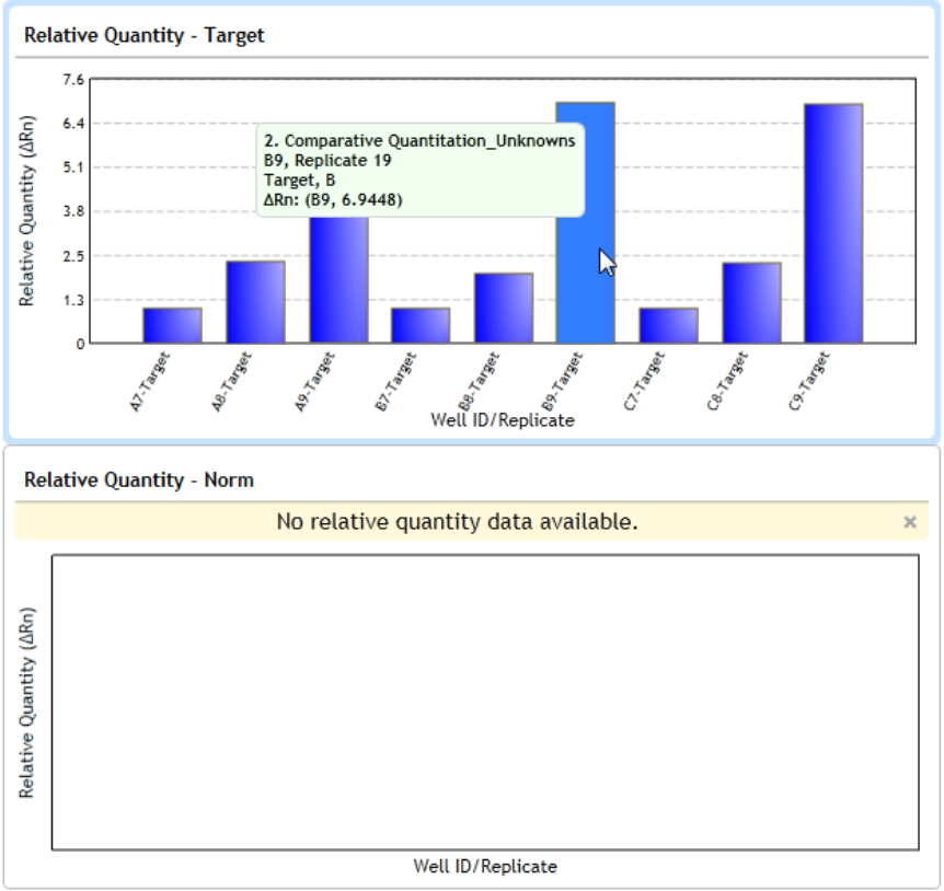
15 “How-To” Examples for Multiple Experiment Analysis Projects
Example 2
319 Agilent Aria Real-Time PCR Program

Agilent Technologies
16
Help for the Aria ET (Electronic
Tracking) Software
Overview of the Aria ET software 321
Open an experiment in the Aria ET software 323
Import and export experiments in the Aria ET software 326
Import experiments into the database 326
Export experiments from the database 326
Lock or log out of the Aria ET software 328
Lock the program 328
Log out of the program 328
Change your password in the Aria ET software 330
Create a multiple experiment analysis project in the Aria ET software 331
Manage users in the Aria ET software 332
Set account properties for all users 332
Manage user accounts 335
Archive and restore experiments in the Aria ET software 339
Archive experiments 339
Restore experiments 341
View audit trails and system logs in the Aria ET software 343
View the audit trail logs 343
View the system logs 346
Add and remove databases in the Aria ET software 348
Add an Aria ET database 349
Remove an Aria ET database 350
View transaction logs in the Aria ET software 352
View transaction logs for primary database 352
View transaction logs for an archive database 353
16 Help for the Aria ET (Electronic Tracking) Software
Overview of the Aria ET software
321 Agilent Aria Real-Time PCR Program
Overview of the Aria ET software
Agilent offers the Aria ET (Electronic Tracking) software component, an
optional upgrade providing security features such as user authentication,
database data storage, and audit trail records. For instructions on
installing the ET version of the Aria software, see the AriaMx/AriaDx
Real- Time PCR System Setup and User's Guide.
If you are running the Aria ET software component, you have access to
the following electronic tracking functions:
• Controlled access to the Aria software through identification of all
application administrators and users, each with a unique username and
encrypted password
• Controlled database access through identification of all databases using
a unique user ID and encrypted password
• Experiment storage, retrieval, and deletion to/from defined database(s)
• Chronological and permanent audit trail recording of administrator and
user actions that create, modify, or delete experiments, as well as error
recording
• Database management, including adding, removing, and switching
databases (switching databases is available at login)
• Controlled access to a defined database through administrator and user
management
• Report generation for audit trail, user account, and error logs
• Report generation for experiment results with electronic signature
(e- signature)
The help topics listed below provide information and instructions on using
the program features that are unique to the ET component.
“Open an experiment in the Aria ET software” on page 323
“Import and export experiments in the Aria ET software” on page 326
“Lock or log out of the Aria ET software” on page 328
“Change your password in the Aria ET software” on page 330
“Create a multiple experiment analysis project in the Aria ET software” on
page 331
Help for the Aria ET (Electronic Tracking) Software 16
Overview of the Aria ET software
Agilent Aria Real-Time PCR Program 322
For administrators, the following help topics provide information on
administrative functions.
“Manage users in the Aria ET software” on page 332
“Archive and restore experiments in the Aria ET software” on page 339
“View audit trails and system logs in the Aria ET software” on page 343
“Add and remove databases in the Aria ET software” on page 348
“View transaction logs in the Aria ET software” on page 352

16 Help for the Aria ET (Electronic Tracking) Software
Open an experiment in the Aria ET software
323 Agilent Aria Real-Time PCR Program
Open an experiment in the Aria ET software
The Aria ET program tracks the actions taken on a post- run experiment
using a primary database with controlled access. If the experiment you
want to open is stored in the primary database, you can open it directly
from the database. If you want to open a post- run experiment that is
saved to a file system (i.e., a local or network folder), you first must
import the experiment into the database. The instructions in this help
topic describe how to open experiments from the primary database. See
“Import and export experiments in the Aria ET software” on page 326 for
instructions on importing experiments.
Open an experiment
You can open an experiment using multiple approaches. When you open
an experiment, you have the option to open the latest snapshot of the
experiment (i.e., the most recent version) or an earlier snapshot of the
experiment. Refer to the image below for an explanation of how the
program organizes experiments and snapshots in its browsers.
Open the latest snapshot of an experiment
You can open the most recent version of an experiment using multiple
approaches.
To open the latest snapshot of an experiment from the Getting Started
screen:
1 Click the icon to the right of the tabs to open a new tab.
The new tab opens to the Getting Started screen.
2 Click one of the options under Saved:

Help for the Aria ET (Electronic Tracking) Software 16
Open an experiment in the Aria ET software
Agilent Aria Real-Time PCR Program 324
• To open an existing experiment that you recently accessed, click
Recently Opened. In the bottom panel of the screen, under
Database, is a list of post- run experiments that you have recently
opened. Double- click the experiment you want to open. The program
opens the experiment to the Plate Setup screen.
• To browse to the folder of the experiment, click Browse Database.
The Browse Database dialog box opens with a list of all experiments
in the primary database, organized by user (see image above). Click
the experiment name (not a snapshot below an experiment) to select
it. Then, click Open. The dialog box closes and the program opens
the experiment to the Plate Setup screen.
To open the latest snapshot of an experiment from the File menu:
1 From the toolbar, click File > Open.
The Open Experiment dialog box opens with a list of all experiments in
the primary database, organized by user (see image above).
2 Click the experiment name (not a snapshot below an experiment) to
select it. Then, click Open. The dialog box closes and the program
opens the experiment to the Plate Setup screen.
Open an earlier snapshot of an experiment
You can open a previous snapshot of an experiment using multiple
approaches.
To open an earlier snapshot of an experiment from the Getting Started
screen:
1 Click the icon to the right of the tabs to open a new tab.
The new tab opens to the Getting Started screen.
2 Under Saved, click Browse Database. The Browse Database dialog box
opens with a list of all experiments in the primary database, organized
by user (see image above). Expand the node for the desired experiment
to view the snapshots available for the experiment.
The date and time stamp for the snapshot are listed in the Date
column.
3 Click a snapshot to select it, then click Open. The dialog box closes and
the program opens the experiment to the Plate Setup screen.
16 Help for the Aria ET (Electronic Tracking) Software
Open an experiment in the Aria ET software
325 Agilent Aria Real-Time PCR Program
To open an earlier snapshot of an experiment from the File menu:
1 From the toolbar, click File > Open.
The Open Experiment dialog box opens with a list of all experiments in
the primary database, organized by user (see image above).
2 Expand the node for the desired experiment to view the snapshots
available for the experiment.
The date and time stamp for the snapshot are listed in the Date
column.
3 Click a snapshot to select it, then click Open. The dialog box closes and
the program opens the experiment to the Plate Setup screen.
Help for the Aria ET (Electronic Tracking) Software 16
Import and export experiments in the Aria ET software
Agilent Aria Real-Time PCR Program 326
Import and export experiments in the Aria ET software
The Aria ET software tracks the actions taken on a post- run experiment
using a primary database with controlled access. If you want to open a
post- run experiment that is saved to a local or network folder, you first
must import the experiment into the database. Similarly, if you want to
make an experiment available outside of the database, you must first
export it to a local or network folder.
Import experiments into the database
Importing a post- run experiment into the database creates a controlled
copy of the experiment and makes it available for opening in the Aria ET
program.
To import an experiment from a folder into the database:
1 From the toolbar, click File > Import From File System.
The Open dialog box opens.
2 Browse to the folder location of the experiment. Select the experiment
and click Open.
The dialog box closes. The program creates a copy of the experiment
and saves it to the primary database.
You can now open the experiment as described in “Open an experiment
in the Aria ET software” on page 323.
Export experiments from the database
Exporting an experiment creates an uncontrolled copy of the experiment.
You may need to export an experiment in order to make it available for
viewing to users outside your network.

16 Help for the Aria ET (Electronic Tracking) Software
Import and export experiments in the Aria ET software
327 Agilent Aria Real-Time PCR Program
To export an experiment from the database to a folder:
1 From the toolbar, click File > Export To File System.
The Export Experiments dialog box opens, listing all experiments in the
primary database, organized by user.
2 Mark the check box for the experiment or snapshot that you want to
export. Marking the experiment will export all snapshots of the
experiment. Marking a snapshot will export only that snapshot. The
date stamp for the snapshots are noted in the Date column.
3 Click Browse.
The Browse For Folder dialog box opens.
4 Browse to the folder where you want to save the exported experiments.
Select the folder and click Open.
The Browse For Folder dialog box closes and the file path for the
selected folder is listed in the Export To Folder field on the Export
Experiments dialog box.
5 Click Export.
The dialog box closes. The program creates a copy of the experiment
and saves it to the specified folder. The file name of the exported
experiment includes a date and time stamp.
Help for the Aria ET (Electronic Tracking) Software 16
Lock or log out of the Aria ET software
Agilent Aria Real-Time PCR Program 328
Lock or log out of the Aria ET software
When the Auto lockout feature is enabled, the program automatically locks
and requires users to re- enter their password if the program is idle for
longer than a set period of time (60 minutes is the default). You can also
lock the program, or log out completely. For example, if you need to step
away from your computer, or need to secure it for any reason, you may
want to lock the program or log out.
Lock the program
Locking the program makes that session of the program inaccessible
without logging out the currently logged- in user. To unlock the program,
users must re- enter the user password. Only the logged- in user or an
administrator can unlock a locked session of the program.
To lock the program:
• From the toolbar, click File > Lock.
The program locks and the Unlock dialog box opens.
To unlock the program:
1 In the Password field of the Unlock dialog box, type the password for
the logged- in user. Alternatively, if you are an administrator, type your
administrator username and password into the fields.
2 Click Login.
Log out of the program
Logging out of the program logs out the currently logged- in user. Any user
can log back in after the current user logs out.
To log out of the program:
• From the toolbar, click File > Logout.
The program logs out the current user and the Login dialog box opens.
16 Help for the Aria ET (Electronic Tracking) Software
Lock or log out of the Aria ET software
329 Agilent Aria Real-Time PCR Program
To log in to the program:
1 In the Login dialog box, type your username and password into the
fields.
2 Click Login.

Help for the Aria ET (Electronic Tracking) Software 16
Change your password in the Aria ET software
Agilent Aria Real-Time PCR Program 330
Change your password in the Aria ET software
By default, the program automatically prompts users to reset the password
for their account every 90 days. However, users can change the password
for their Aria ET account at any time using the instructions provided here.
To change the password for your Aria ET user account:
1 From the toolbar, click File > Logout.
The program logs you out and the Login dialog box opens.
2 In the Login dialog box, click Change Password.
The Change Password dialog box opens.
3 Type your Username, Old Password, and New Password into the fields.
Type the new password again into the Confirm Password field.
Passwords must be 6- 15 alphanumeric characters in length and include
at least one number.
4 Click OK.
The Change Password dialog box closes and you are returned to the
Login dialog box.
5 Type your Username and Password into the fields, using your new
password.
6 Click Login.
NOTE
Administrators can reset the password for any user account at any time. See
“Change a user's password” on page 337 for instructions.
16 Help for the Aria ET (Electronic Tracking) Software
Create a multiple experiment analysis project in the Aria ET software
331 Agilent Aria Real-Time PCR Program
Create a multiple experiment analysis project in the Aria ET software
Multiple experiment analysis (MEA) is a feature in the Aria software that
allows you to display and analyze the results from two or more post- run
experiments together in a single file called a project. See “Overview of
multiple experiment analysis” on page 270 for a description of MEA.
Although the ET version of the Aria software allows you to create MEA
projects and analyze the data in those projects, the projects are not stored
in a database and the program does not electronically track the actions
taken on projects.
To create an MEA project in the Aria ET program:
1 Export the post- run experiments to be added to the project from the
database to a file system. See “Export experiments from the database”
on page 326.
2 Create the project in the same manner as that used for the standard
version of the Aria software. See “Create an MEA project” on page 275.
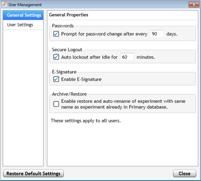
Help for the Aria ET (Electronic Tracking) Software 16
Manage users in the Aria ET software
Agilent Aria Real-Time PCR Program 332
Manage users in the Aria ET software
If you are running the electronic tracking (ET) version of the Aria
software, and you logged in using an administrator account, you have
access to User Management dialog box for managing users and account
settings.
To open the User Management dialog box: At the top of the program
window, click Admin > User Management.
Set account properties for all users
The General Settings tab of the User Management dialog box has settings
that apply to all users on the database.
16 Help for the Aria ET (Electronic Tracking) Software
Manage users in the Aria ET software
333 Agilent Aria Real-Time PCR Program
Set the password expiration properties
You can change how frequently the program prompts users to reset their
passwords. You can also eliminate password expirations so that the
program no longer requires users to reset their passwords after a set
period of time.
To change the password expiration time:
1 Open the User Management dialog box to the General Settings tab.
2 Under Passwords, make sure the check box is marked, and in the field,
type the number of days that you want the expiration time to be. The
default is 90 days, which means that the program automatically
prompts users to reset their password every 90 days.
3 Click Close to close the dialog box and apply your changes.
To eliminate password expirations:
1 Open the User Management dialog box to the General Settings tab.
2 Under Passwords, clear the check box next to Prompt for password
change every [x] days.
3 Click Close to close the dialog box and apply your changes.
Users will no longer be prompted to change their passwords after a set
period of time.
Set the auto lockout properties
You can change the length of idle time required before the program
automatically locks and requires users to re- enter their password. You can
also disable the automatic lockout feature completely.
To change the length of idle time required before automatic lockout:
1 Open the User Management dialog box to the General Settings tab.
2 Under Secure Logout, make sure the check box is marked, and in the
field, type the number of minutes for the desired idle time. The default
is 60 minutes, which means that the program automatically locks after
60 minutes of inactivity.
3 Click Close to close the dialog box and apply your changes.
Help for the Aria ET (Electronic Tracking) Software 16
Manage users in the Aria ET software
Agilent Aria Real-Time PCR Program 334
To disable automatic logout:
1 Open the User Management dialog box to the General Settings tab.
2 Under Secure Logout, clear the check box next to Auto lockout after
idle for [x] minute.
3 Click Close to close the dialog box and apply your changes.
The program no longer locks after a period of inactivity.
Disable or enable the e-signature requirement
By default, the program requires users to re- enter their password before
allowing them to print or export an experiment report. This step serves as
an electronic signature (e- signature) to verify that the logged- in user
approves of the report. The User Management dialog box has tools for
disabling and enabling the e- signature requirement.
To disable e- signature:
1 Open the User Management dialog box to the General Settings tab.
2 Under E- Signature, clear the check box.
3 Click Close to close the dialog box and apply your changes.
The program no longer requires an e- signature to print or export
reports.
To enable e- signature:
1 Open the User Management dialog box to the General Settings tab.
2 Under E- Signature, mark the check box.
3 Click Close to close the dialog box and apply your changes.
The program now requires an e- signature to print or export reports.
Enable or disable auto-renaming of restored experiments
The auto- renaming feature is for the automatic renaming of experiments
restored to the primary database. If you restore an experiment to the
primary database, but the database already contains an experiment of the
same name, auto- renaming appends a bracketed number to the name of
the restored experiment. When auto- renaming is disabled, you cannot
restore an experiment if the primary database already contains an
experiment of the same name.
16 Help for the Aria ET (Electronic Tracking) Software
Manage users in the Aria ET software
335 Agilent Aria Real-Time PCR Program
To enable auto- renaming:
1 Open the User Management dialog box to the General Settings tab.
2 Under Archive/Restore, mark the check box.
3 Click Close to close the dialog box and apply your changes.
Auto- renaming is now enabled.
To disable auto- renaming:
1 Open the User Management dialog box to the General Settings tab.
2 Under Archive/Restore, clear the check box.
3 Click Close to close the dialog box and apply your changes.
Auto- renaming is now disabled.
Manage user accounts
The User Settings tab of the User Management dialog box has tools for
creating and editing user accounts.

Help for the Aria ET (Electronic Tracking) Software 16
Manage users in the Aria ET software
Agilent Aria Real-Time PCR Program 336
Create a user account
Create user accounts for each user who needs to log in to the Aria ET
program and access the database.
To create a user account:
1 Open the User Management dialog box to the User Settings tab.
2 Click Create User.
The fields in the bottom panel of the dialog box (e.g., Username, Full
Name, etc.) become editable.
3 Complete all fields.
Username: Type a username for the new account
Full Name: Type the name (first and last) of the person who will be
using the account
16 Help for the Aria ET (Electronic Tracking) Software
Manage users in the Aria ET software
337 Agilent Aria Real-Time PCR Program
Password: Type a password for the account (must be 6- 15
alphanumeric characters in length and include at least one number)
Retype Password: Type the same password you entered above
4 Next to User Type, select the access privileges for the new user
• Select Administrator to give the user administrator privileges
• Select User to give the user standard privileges
Administrator privileges include managing user accounts and databases,
archiving and restoring experiments, and viewing audit trails and
transaction logs.
5 Click Close to close the dialog box and apply your changes.
Disable or enable a user account
Once created, you cannot delete a user account but you can disable the
account to prevent the user from being able to log in to the Aria ET
program. You can also re- enable a disabled user account.
To disable a user account:
1 Open the User Management dialog box to the User Settings tab.
2 In the table, locate the account that you want to disable and clear the
check box in the Enable column.
3 Click Close to close the dialog box and apply your changes.
To enable a user account:
1 Open the User Management dialog box to the User Settings tab.
2 In the table, locate the account that you want to enable and mark the
check box in the Enable column.
3 Click Close to close the dialog box and apply your changes.
Change a user's password
As an administrator, you can change the password for any user account in
the database.
To change a password:
1 Open the User Management dialog box to the User Settings tab.
2 In the table, click on the row for the desired user account to select it.
Help for the Aria ET (Electronic Tracking) Software 16
Manage users in the Aria ET software
Agilent Aria Real-Time PCR Program 338
The account information for the selected user is displayed in the bottom
panel of the dialog box.
3 Click Change Password.
The Password and Retype Password fields become editable.
4 In the Password field, type a new password for the account. Passwords
must 6- 15 alphanumeric characters in length and contain a number.
5 In the Retype Password field, type the password again.
6 Click Save to save the new password.
Print or export the user account table
You can print a copy of the table that appears on the User Settings tab of
the User Management dialog box. You can also export a copy of the table
to Microsoft Excel.
To print the user account table:
1 Open the User Management dialog box to the User Settings tab.
2 Click Print.
The Print dialog box opens.
3 Select a printer and click Print.
The program prints a copy of the table.
To export the user account table to Excel:
1 Open the User Management dialog box to the User Settings tab.
2 Click Export to Excel.
Excel launches with a copy of the user account table displayed.
3 Save the Excel file, if desired.

16 Help for the Aria ET (Electronic Tracking) Software
Archive and restore experiments in the Aria ET software
339 Agilent Aria Real-Time PCR Program
Archive and restore experiments in the Aria ET software
If you are running the electronic tracking (ET) version of the Aria
software, and you logged in using an administrator account, you can
archive experiments to an archive database and restore previously
archived experiments.
To open the Archive dialog box: At the top of the program window, click
Admin > Archive Experiments.
To open the Restore dialog box: At the top of the program window, click
Admin > Restore Experiments.
Archive experiments
The Archive dialog box has tools for archiving experiments and creating
new archive databases. Archiving an experiment requires moving it from
the primary database to an archive database. Once archived, users cannot
work in an experiment unless an administrator restores it.
NOTE
In order to archive or restore experiments, your PC must be running MSDTC
service. See the AriaMx/AriaDx Setup and User's Guide for instructions on
configuring and starting the MSDTC service.

Help for the Aria ET (Electronic Tracking) Software 16
Archive and restore experiments in the Aria ET software
Agilent Aria Real-Time PCR Program 340
Create an archive database
Before you archive an experiment, you may wish to create a new archive
database. Creating an archive database makes it available in the Select
Archive Database drop- down list in the Archive dialog box.
To create an archive database:
1 Open the Archive dialog box (Admin > Archive Experiments).
2 In the Select Archive Database drop- down list, click Create new.
The Create Archive Database dialog box opens.
3 In the Server Name drop- down list, select the appropriate server.
4 In the Password field, type your SQL Server password.
5 In the Database name field, type a name for the new archive database.
6 Click Create.
A message box opens confirming the creation of the new database.
Click OK to close the message box.

16 Help for the Aria ET (Electronic Tracking) Software
Archive and restore experiments in the Aria ET software
341 Agilent Aria Real-Time PCR Program
Archive experiments
To archive an experiment:
1 Open the Archive dialog box (Admin > Archive Experiments).
2 In the Select Archive Database drop- down list, select the desired
archive database.
3 In the table, mark the check box in the Archive column for the
experiments that you want to archive.
To search for an experiment, type a search term into the Search field at
the top of the dialog box.
To archive all experiments, mark Select All Experiments to Archive at
the bottom of the dialog box.
4 Click Archive.
A message box opens confirming the number of experiments that the
program successfully archived.
Restore experiments
Using the Restore dialog box, you can take archived experiments out of
the archive database and restore them to their original primary database
or a different primary database. Restoring experiments makes them
available for further editing and analysis.
NOTE
In order to archive or restore experiments, your PC must be running MSDTC
service. See the AriaMx/AriaDx Setup and User's Guide for instructions on
configuring and starting the MSDTC service.
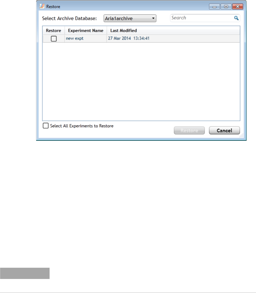
Help for the Aria ET (Electronic Tracking) Software 16
Archive and restore experiments in the Aria ET software
Agilent Aria Real-Time PCR Program 342
To restore an archived experiment:
1 Open the Restore dialog box (Admin > Restore Experiments).
2 In the Select Archive Database drop- down list, select the desired
archive database.
3 In the table, mark the check box in the Archive column for the
experiments that you want to archive.
To search for an experiment, type a search term into the Search field at
the top of the dialog box.
To restore all experiments, mark Select All Experiments to Restore at
the bottom of the dialog box.
4 Click Restore.
A message box opens confirming the number of experiments that the
program successfully restored.
NOTE
In order to archive or restore experiments, your PC must be running MSDTC
service. See the AriaMx/AriaDx Setup and User's Guide for instructions on
configuring and starting the MSDTC service.
16 Help for the Aria ET (Electronic Tracking) Software
View audit trails and system logs in the Aria ET software
343 Agilent Aria Real-Time PCR Program
View audit trails and system logs in the Aria ET software
If you are running the electronic tracking (ET) version of the Aria
software, and you logged in using an administrator account, you have
access to the audit trails and system logs that are available in the Log
Viewer dialog box.
To open the Log Viewer dialog box: At the top of the program window,
click Admin > Log Viewer.
View the audit trail logs
The audit trail logs show all snapshots of an experiment. The program
saves a new snapshot of an experiment each time a user performs a
tracked action in the experiment (e.g., changing an analysis setting). For
each snapshot, the logs indicate the user who performed the action, the
date and time of the action, and a description of the action.

Help for the Aria ET (Electronic Tracking) Software 16
View audit trails and system logs in the Aria ET software
Agilent Aria Real-Time PCR Program 344
Open and navigate the audit trail logs
The audit trail logs show all available snapshots for each experiment,
organized first by username then by experiment name.
To open the audit trail logs and navigate its contents:
1 Open the Log Viewer dialog box (Admin > Log Viewer).
2 Next to Log, select Audit Trail Logs (if not already selected).
The table at the top of the dialog box lists the users on the database,
with experiments listed under each user, and previous snapshots for the
experiment listed below (as described in the image below).

16 Help for the Aria ET (Electronic Tracking) Software
View audit trails and system logs in the Aria ET software
345 Agilent Aria Real-Time PCR Program
3 Click on an experiment name or snapshot in the table. (To help locate
a particular experiment, type a search term into the Search field at the
top of the dialog box.)
The table at the bottom of the dialog box shows
all actions taken by
the user for a selected snapshot (if you selected a snapshot) or
for the entire experiment
(if you selected an experiment).
Print or export the audit trail logs
You can print a copy of the table that appears at the bottom of the Log
View - Audit Trail Logs dialog box. You can also export a copy of the
table to Microsoft Excel.
To print the table:
1 Open the Log Viewer dialog box to the Audit Trail Logs.
2 In the table at the top of the dialog box, select an experiment or
snapshot (see Open and navigate the audit trail logs, above, for
detailed instructions).
3 Click Print.
The Print dialog box opens.
4 Select a printer and click Print.
The program prints a copy of the table.

Help for the Aria ET (Electronic Tracking) Software 16
View audit trails and system logs in the Aria ET software
Agilent Aria Real-Time PCR Program 346
To export the table to Excel:
1 Open the Log Viewer dialog box to the Audit Trail Logs.
2 In the table at the top of the dialog box, select an experiment or
snapshot (see Open and navigate the audit trail logs, above, for
detailed instructions).
3 Click Export to Excel.
Excel launches with a copy of the table displayed.
4 Save the Excel file, if desired.
View the system logs
The system logs show the actions taken to manage user account
information as well as any failed login attempts. For each action item, the
logs indicate the user who performed the action, the date and time of the
action, and a description of the action. The system logs also show the
total number of experiments that have been archived or restored and any
failed attempts to archive or restore an experiment. For failed archive or
restore attempts, the logs list the experiment name and the failure error
message.
16 Help for the Aria ET (Electronic Tracking) Software
View audit trails and system logs in the Aria ET software
347 Agilent Aria Real-Time PCR Program
Open the system logs
To open the system logs:
1 Open the Log Viewer dialog box (Admin > Log Viewer).
2 Next to Log, select System Logs.
The table displays list system actions in chronological order.
Print or export the system logs
You can print a copy of the system logs table or export a copy to
Microsoft Excel.
To print the system logs:
1 Open the Log Viewer dialog box to the System Logs.
2 Click Print.
The Print dialog box opens.
3 Select a printer and click Print.
The program prints a copy of the table.
To export the system logs to Excel:
1 Open the Log Viewer dialog box to the System Logs.
2 Click Export to Excel.
Excel launches with a copy of the table displayed.
3 Save the Excel file, if desired.
Help for the Aria ET (Electronic Tracking) Software 16
Add and remove databases in the Aria ET software
Agilent Aria Real-Time PCR Program 348
Add and remove databases in the Aria ET software
If you are running the electronic tracking (ET) version of the Aria
software, and you logged in using an administrator account, you can
control which primary and archive databases are available to users on
your system.
To open the Add Database dialog box: At the top of the program
window, click Admin > Add Database.
To open the Remove Database dialog box: At the top of the program
window, click Admin > Remove Database.
Adding a database through the Add Database dialog box does not create a
new database; it only makes the database available for use by the Aria ET
program on your PC by adding a reference to the database. Similarly,
removing a database through the Remove Database dialog box does not
delete a database; it only makes the database unavailable for use by the
Aria ET program on your PC by removing a reference to the database.
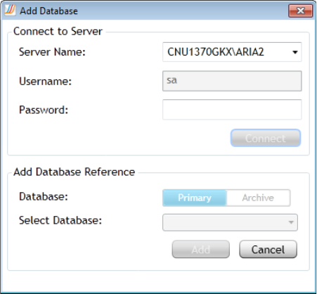
16 Help for the Aria ET (Electronic Tracking) Software
Add and remove databases in the Aria ET software
349 Agilent Aria Real-Time PCR Program
Add an Aria ET database
The Add Database dialog box has tools for adding primary and archive
databases.
Add a primary database
Each time a user launches the Aria ET program, the Login dialog box
opens, prompting the user to login to an Aria ET database. Using the Add
Database dialog box, you can add a database to the list of available
databases that appears on the Login dialog box.
To add a primary database:
1 Open the Add Database dialog box (Admin > Add Database).
The program searches your local machine and network to identify
available servers.
2 In the Server Name drop- down list, select the appropriate server.
3 Type your SQL Server password into the Password field.
4 Click Connect.
5 Next to Database, make sure the Primary option is selected.
6 In the Select Database drop- down, select the desired database. This
drop- down lists all primary databases available on the server.
Help for the Aria ET (Electronic Tracking) Software 16
Add and remove databases in the Aria ET software
Agilent Aria Real-Time PCR Program 350
7 Click Add.
The dialog box closes and the database is listed in the Login dialog box
the next time a user launches the program.
Add an archive database
When you archive an experiment, the Archive dialog box includes a
drop- down list of available archive database. You can use the tools on the
Add Database dialog box to add an archive database to that drop- down
list.
To add an archive database:
1 Open the Add Database dialog box (Admin > Add Database).
The program searches your local machine and network to identify
available servers.
2 In the Server Name drop- down list, select the appropriate server.
3 Type your SQL Server password into the Password field.
4 Click Connect.
5 Next to Database, select Archive.
6 In the Select Database drop- down, select the desired database. This
drop- down lists all archive databases available on the server.
7 Click Add.
The dialog box closes and the database is listed in the Archive dialog
box the next time a user archives an experiment.
Remove an Aria ET database
If you have previously added databases, and have multiple databases
available on your system, you can remove a database. Removing a primary
database makes it no longer available in the Login dialog box that opens
when users launch the Aria ET program. Removing an archive database
makes it no longer available when users archive or restore an experiment.

16 Help for the Aria ET (Electronic Tracking) Software
Add and remove databases in the Aria ET software
351 Agilent Aria Real-Time PCR Program
To remove a database:
1 Open the Remove Database dialog box (Admin > Remove Database).
2 Next to Database, select Primary to remove a primary database or
Archive to remove an archive database.
The program populates the table with all available primary databases (if
Primary is selected) or all available archive databases (if Archive is
selected).
3 In the table, mark the check box in the Remove column for the
database that you want to remove. Note that you cannot mark the
check box for the currently logged- in database (the row is grayed out in
the table).
4 Click Remove.
The database is removed from the table.
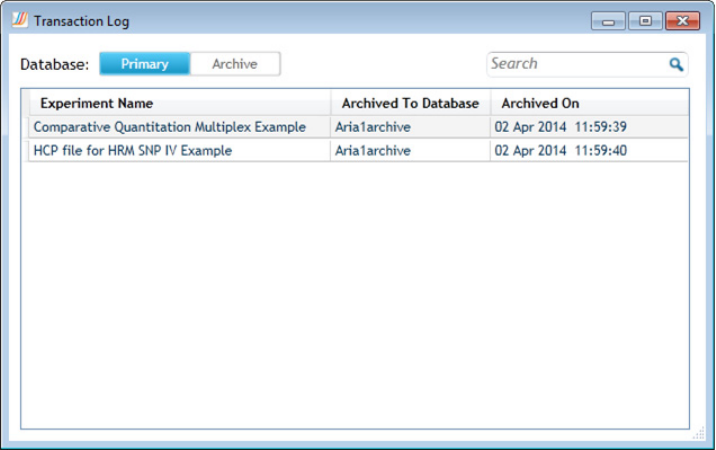
Help for the Aria ET (Electronic Tracking) Software 16
View transaction logs in the Aria ET software
Agilent Aria Real-Time PCR Program 352
View transaction logs in the Aria ET software
If you are running the electronic tracking (ET) version of the Aria
software, and you logged in using an administrator account, you can view
the transaction logs, which track archiving and restoring activities.
To open the Transaction Log dialog box: At the top of the program
window, click Admin > Transaction Log.
View transaction logs for primary database
The Transaction Log dialog box can display all the experiments that have
been archived from the primary database. Note that the logs do not
include archived experiments that were later restored to their original
primary database.
To view the log of archive transactions:
1 Open the Transaction Logs dialog box (Admin > Transaction Log).
2 Next to Database, select Primary (if not already selected).
16 Help for the Aria ET (Electronic Tracking) Software
View transaction logs in the Aria ET software
353 Agilent Aria Real-Time PCR Program
The table lists the experiments that have been archived (Experiment
Name column), which database they were archived to (Archived To
Database column), and the date and time that they were archived
(Archived On column).
To help locate a particular experiment, type a search term into the
Search field at the top of the dialog box.
View transaction logs for an archive database
The Transaction Log dialog box can display all the experiments that have
been restored from an archive database to the primary database.
To view the log of restoration transactions:
1 Open the Transaction Logs dialog box (Admin > Transaction Log).
2 Next to Database, select Archive.
3 In the Select Archive Database drop- down list, select the archive
database for which you want to view the logs.
The table lists contains the following columns:
• Experiment Name: experiments that have been archived/restored
• Archived From Database: primary database from which the
experiment was archived
• Archived On: date and time that the experiment was archived
• Restored To Database: primary database to which the experiment
was restored
• Restored On: date and time that the experiment was restored
To help locate a particular experiment, type a search term into the
Search field at the top of the dialog box.

17 Reference Help and Troubleshooting & Support
QPCR Glossary
355 Agilent Aria Real-Time PCR Program
QPCR Glossary
Experiment Type and QPCR Detection Chemistry Terms
Quantitative PCR Experiment Type: Experiments of this type typically
use a standard curve to quantitate the amount of target present in an
unknown sample with high accuracy using a fluorescently- labeled probe or
double- stranded DNA- binding dye for detection. A series of Standard
samples, containing dilutions of a known amount of target, are amplified
to generate a curve that relates the initial quantity of the specific target to
the Cq. The standard curve is then used to derive the initial template
quantity in Unknown wells based on their Cq values. This method is
sometimes referred to as absolute quantitation or as standard- curve
quantitation in the literature. This experiment type is also useful for
primer/probe optimization experiments in the absence of a standard curve.
Comparative Quantitation Experiment Type: This experiment type is a
form of relative quantitation, comparing the levels of a target gene in test
samples (referred to as Unknowns) relative to a sample of reference
(referred to as the calibrator). For example, the calibrator sample might
contain RNA from untreated cells, while the Unknowns might contain RNA
from cells treated with different experimental agents. This experiment type
provides an efficient method for comparing levels of RNA or DNA across
samples when information about the absolute amounts of target in any
sample is not required. This method is used for establishing relative
quantitation without the need for repeatedly performing a dilution series
standard curve.
Allele Discrimination Experiment Type, Fluorescence Probe: In this
experiment type, two fluorescent probes labeled with two spectrally
distinct dyes are used to discriminate between the two alleles and,
subsequently, determine the genotype of a sample. For example, if the
program detects amplification in an unknown DNA sample for the dye
identifying the wild- type allele but not for the dye identifying a mutant
allele, the program designates the sample as wild- type homozygous.
Allele Discrimination Experiment Type, DNA Binding Dye Including
HRM: When using this experiment type, you set up the experiment to
amplify all alleles in the same well using the same set of primers, and the
program detects all alleles using the same double- stranded DNA- binding
dye (such as SYBR Green or EvaGreen dye). The thermal profile includes
Reference Help and Troubleshooting & Support 17
QPCR Glossary
Agilent Aria Real-Time PCR Program 356
a high- resolution melt (HRM) segment so that melt curves of the targets
can be generated. Even DNA amplicons that differ in sequence by only a
single nucleotide will yield slightly different melt curves. An Allele
Discrimination experiment that uses HRM analysis for allele discrimination
should include positive control samples for each base pair possibility at
the SNP location (homozygous as well as heterozygous positive control
samples).
Reference Dye: Passive dye used for normalization of the fluorescence
signal of the reporter dye or fluorophore. The reference dye fluoresces at
a constant level during the reaction.
Reporter Dye: Fluorescent dye that increases in fluorescence signal as the
amount of PCR product increases.
Normalizer: Available in Comparative Quantitation experiments and User
Defined experiments, the normalizer is a target that is known to be
unaffected by the experimental treatment under investigation, and thus is
found in equal quantity across all template samples. Data from the
normalizer target is used to normalize the fluorescence signal of the
targets of interest.
FRET Chemistry (Fluorescence Resonance Energy Transfer): In FRET
chemistry, the excitation of a donor fluorescent dye is transferred to a
receptor dye, leading to the fluorescence of the acceptor dye instead of
the donor dye. The transfer is possible only if the two dyes are in close
proximity.
TaqMan Probes: These are linear fluorescently- labeled hydrolysis probes
that can be used to monitor PCR product formation either during or after
the amplification process. As the DNA polymerase extends the upstream
primer and encounters the downstream probe, the exonuclease activity of
the polymerase cleaves the probe. In this event, the reporter fluorophore
is released into the reaction solution and is able to fluoresce.
Quencher: A quencher is a moiety that absorbs the energy of the reporter
dye in its excited state. The quencher can emit its own fluorescence signal
(TAMRA) or emit no fluorescence signal (DABCYL, BHQ).
17 Reference Help and Troubleshooting & Support
QPCR Glossary
357 Agilent Aria Real-Time PCR Program
Well-Types
Unknown: Contains a complete reaction mixture including a test template
that contains an unknown amount of the specific target.
Buffer: Contains only buffer, used to monitor the background fluorescence
attributable to the buffer.
NAC: No amplification control; contains all reaction components except
DNA polymerase.
NPC: No probe control; contains all reaction components except the
fluorescence- labeled probe.
NTC: No template control; contains all reaction components except the
template nucleic acid.
Standard: Contains a complete reaction mixture including a known
concentration of target nucleic acid. Used to generate a standard curve,
which is then used to relate the quantification cycle (Cq) to initial
template quantity in Unknown wells.
No RT: No reverse transcriptase control; contains all QRT- PCR reaction
components except reverse transcriptase.
Allele A+: Available in Allele Discrimination experiments and User
Defined experiments. Contains a complete reaction mixtures with a
template sample that is a positive control for homozygous allele A.
Allele B+: Available in Allele Discrimination experiments and User
Defined experiments. Contains a complete reaction mixtures with a
template sample that is a positive control for homozygous allele B.
Mixed+: Available in Allele Discrimination experiments and User Defined
experiments. Contains a complete reaction mixtures with a template
sample that is a positive control for mixture of allele A and allele B.
Calibrator: Available in Comparative Quantitation experiments and User
Defined experiments as the reference sample to which Unknowns are
compared. Contains a complete reaction mixture including a characterized
target. The level of a target- of- interest in the Calibrator wells is set to
1.0 for comparison to the relative quantities in unknown samples.
Reference Help and Troubleshooting & Support 17
QPCR Glossary
Agilent Aria Real-Time PCR Program 358
Analysis Terms
Standard Curve: The Standard Curve is a plot of the Cq (quantification
cycle) on the Y- axis versus the initial template quantity added to standard
wells on the X- axis. A best- fit curve is displayed for each dye with data
collected in Standard wells.
Amplification Plot: The Amplification Plots view shows a plot of
fluorescence versus cycles for each plateau on which data are gathered.
Initial Template Quantity: Provides interpolated quantities of template
added to Unknown wells before thermal cycling. The quantities are
interpolated from a standard curve based on the calculated Cq values
determined for the known quantities of template in the Standard wells.
Baseline Correction: For each well and each path the raw fluorescence
data are fit over the specified range of cycles using a linear least mean
squares algorithm to produce a baseline. The value of the baseline
function is calculated for every cycle and subtracted from the raw
fluorescence to produce the baseline corrected fluorescence (dR).
Quantification Cycle (Cq): The Cq is the cycle at which fluorescence is
determined to be statistically significant above background signal
contributed by the fluorescently labeled oligonucleotides within the PCR
reaction. The quantification cycle is inversely proportional to the log of
the initial copy number.
Background Cycle Range: The background cycle range specifies the range
of cycles of fluorescence data the program uses to calculate the
background noise level when using the Background- based threshold
algorithm to set the threshold fluorescence. The region specified is
typically in the cycle range before exponential amplification occurs. The
standard deviation of the raw fluorescence for the specified cycles is
calculated and is multiplied by the constant Sigma multiplier for threshold
fluorescence.
Replicates: In the Aria program, the term replicates refers to technical
replicates. Technical replicates are QPCR reaction tubes containing
identical reaction components and set up using a template from the exact
same biological sample source. While biological replicates measure the
variability in the experimental results due to uncontrolled biological
variation from sample to sample, technical replicates are used to measure
the variability in results that is introduced during the process of
experimental setup. Designating replicate wells allows the program to
17 Reference Help and Troubleshooting & Support
QPCR Glossary
359 Agilent Aria Real-Time PCR Program
average results from those wells when the Treat Collectively setting is
used.
Collective Replicate Treatment: Collective replicate treatment causes the
program to analyze all wells with the same replicate symbol as a group,
effectively treating the measurements as all coming from the same well.
Biological Replicates: Biological replicates are template samples that were
isolated independently but from biologically- identical sources (that is,
sources that are genetically identical, are of the same cell type and were
treated identically during experimentation). For example, two samples of
cDNA that were isolated from the same tissue source in two different mice
that were exposed to identical conditions and have the same genotype
would be biological replicates. Biological replicates help you determine the
level of variability in gene expression for your specific experiment that is
due to uncontrolled biological variation from sample to sample. When
setting up the plate for a Comparative Quantitation experiment, you may
designate two or more samples as biological replicates while assigning the
sample names. Samples that are biological replicates are assigned the
same sample name but have different biological replicate ID numbers.
R- squared: The R
2
value is an indication of the fit of the standard curve
to the standard data points plotted. The value will always be between 0
and 1. The closer the value is to 1, the better the fit of the line.
Sigma: Sigma is a measurement of the variability (standard deviation) of
the fluorescence measured from all wells and more than one cycle.
Typically its value is determined from the first few cycles, before the PCR
reaction starts to affect the measurement. The Sigma multiplier is a
user- defined number that is used to multiply by sigma to create a
threshold value for determination of Cq.
p- value: The p- value refers to the probability that the mean of one set of
sample data is different than the mean of another set of sample data. The
first set of sample data is always the control wells in the analysis
selection. When replicates are being treated individually, the second set of
sample data consists of a single well (usually an Unknown well). When
replicates are being treated collectively, the second set of sample data
consists of all of the replicates. If the p- value exceeds the user- specified
confidence level, the well/dye is given a (+) call, whereas if the p- value
does not exceed the user- specified confidence level, the well/target is
given a (- ) call.
Reference Help and Troubleshooting & Support 17
QPCR Glossary
Agilent Aria Real-Time PCR Program 360
Confidence Level: The user- defined confidence level for calls is the
statistical probability required before the algorithm will call amplification
occurrence in a well. The default is 99%.
Multicomponent: Multicomponent is a term used for distinguishing the
contribution that each dye and the background makes to the total
fluorescence spectra detected.

17 Reference Help and Troubleshooting & Support
LIMS File Format for Aria Software
361 Agilent Aria Real-Time PCR Program
LIMS File Format for Aria Software
In order for the experiment data in a LIMS data file to be importable into
the Aria software, the information in the file must follow a specific
format. This topic discusses the format requirements for the LIMS data
file sections that are supported by Aria. These formats must be used in a
LIMS data file that is imported into the program as part of creating a new
experiment.
An Aria- supported LIMS data file can be created by exporting a post- run
experiment to a LIMS data file from within the Aria software. This
approach ensures that the proper format is used. Once exported, you can
edit the file contents as desired. You can also create an Aria- supported
LIMS data file by setting up a text file in Microsoft Excel or another
spreadsheet or text editing program, or by exporting content from a LIMS
software program. If using these approaches, make sure the format of the
file is importable into the Aria software before using it to create a new
experiment.
Verifying proper integration of LIMS functionality, including import and
export of Aria- related data elements, is the responsibility of the end- user.
Plate Setup
To create a new experiment in the Aria software by importing a LIMS
data file, the file must include a Plate Setup section.
The content of the first row of the Plate Setup section needs to be "[Plate
Setup]". The second row needs to contain the headers, separated by a
delimiter. The only headers that are required in order to have a valid
LIMS data file are:
• Well – Enter the well ID, e.g., A1
• Dye – Enter the dye used for target detection
NOTE
When importing a LIMS data file to create a new Aria experiment, the only
required data section is Plate Setup. The other sections are optional, and when
present they will be imported as part of the new Aria experiment creation, but they
are not required in order for the file to be valid and importable.

Reference Help and Troubleshooting & Support 17
LIMS File Format for Aria Software
Agilent Aria Real-Time PCR Program 362
If a single well contains multiple dyes/targets, then include a separate row
for each, as shown in the example image below.
The following headers are also supported for the Plate Setup section:
• Target
• Replicate
• Sample Name
• Well Name
• Well Type – Enter a predefined well type that is supported for the
experiment type (see Chapter 5, “Selecting an Experiment Type” for
descriptions of the available well types in each experiment type)
• Starting Amount – Enter a positive floating number; only imported for
Standard well types
• Normalizer Dye
• Biological Replicate
17 Reference Help and Troubleshooting & Support
LIMS File Format for Aria Software
363 Agilent Aria Real-Time PCR Program
Experiment Setup
An Aria- supported LIMS data file can also include an Experiment Setup
section, which contains information that applies to the entire experiment.
The content of the first row of the Experiment Setup section needs to be
"[Experiment Setup]". The second row can contain any of the following
headers, separated by a delimiter:
• Type – Enter as: Quantitative PCR (DNA Binding Dye including Melt),
Quantitative PCR (Fluorescence Probe), Allele Discrimination (DNA
Binding Dye including High Resolution Melt), Allele Discrimination
(Fluorescence Probe), Comparative Quantitation, or User- Defined
• Name
• Note
• Reference Dye
• Allele A
• Allele B
• Quantity Unit
Thermal Profile
An Aria- supported LIMS data file can also include a Thermal Profile
section, which contains information on the thermal profile.
The content of the first row of the Thermal Profile section needs to be
"[Thermal Profile]". The second row can contain any of the following
headers, separated by a delimiter:
• Segment – Enter a valid segment type; see “Set up the thermal profile”
on page 143
• Plateau – Enter a number 1 through 4 to specify the order of each
plateau within the same segment
• Temperature – Enter temperature in °C from 25.0 to 99.0
• Duration – Enter the duration of the plateau numerically as hh:mm:ss,
from 00:01 to 18:12:15
• Cycle – Enter a positive integer (maximum of 50 for Amplification
segments; maximum of 1 for other segment types)
• DataMarker – Enter No, Plateau, or Ramp

Reference Help and Troubleshooting & Support 17
LIMS File Format for Aria Software
Agilent Aria Real-Time PCR Program 364
• Resolution – Enter 0.5 for normal melt or 2.0 for HRM (for High
Resolution Melt segments, this data field is ignored and 0.2 resolution is
automatically used)
• Soak Time – Enter a positive integer from 3 to 30; only imported for
Melt segments
The subsequent rows in the file contain the identifiers for each column.
Default Optical Module
An Aria- supported LIMS data file can also include a Default Optical
Module section, which contains information on the optical module setup
for the experiment.
The content of the first row of the Default Optical Module section needs to
be "[Default Optical Module]". The second row contains the following
headers, separated by a delimiter:
• Optical Path – Enter a number 1 through 6 to specify the path of each
customized default optical module installed on the instrument
• Optical Dye
The subsequent rows in the file contain the identifiers for each column.
The number of optical modules and the sequence of the optical modules
listed in the file need to match those of the instrument on which you will
run the experiment. If they do not match, you can manually adjust the
modules in the instrument, or, if you transferred the experiment file to
the instrument using a USB drive, you can use the Sync Plate feature on
the Plate Setup screen of the instrument touchscreen.
Threshold Fluorescence
An Aria- supported LIMS data file can also include a Threshold
Fluorescence section, which contains information on the target,
17 Reference Help and Troubleshooting & Support
LIMS File Format for Aria Software
365 Agilent Aria Real-Time PCR Program
fluorescence term, and fluorescence value that will define the threshold
fluorescence during analysis of the post- run experiment data.
The content of the first row of the Threshold Fluorescence section needs
to be "[Threshold Fluorescence]". The second row contains the following
headers, separated by a delimiter:
• TF Target – Enter the target name of the threshold fluorescence target
• TF Term – Enter R, dR, Rn, or dRn
• TF Value – Enter a positive floating number
The subsequent rows in the file contain the identifiers for each column.
Reference Help and Troubleshooting & Support 17
Trademarks
Agilent Aria Real-Time PCR Program 366
Trademarks
SYBR® is a registered trademark of Molecular Probes, Inc.

17 Reference Help and Troubleshooting & Support
Troubleshooting and Support
367 Agilent Aria Real-Time PCR Program
Troubleshooting and Support
Troubleshooting Guide
Observation Suggestion
Unable to install the Aria software You will be unable to install the software if the account that was used to
log in to the PC does not have administrative rights. Log in under an
account with admin rights. If the computer is on a network, you may have
to contact your IT department.
Unable to open post-run Aria files
(*.amxd or *.adxd) on the
PC-installed Aria software
Make sure that the Aria software is installed on a PC running the Windows
operating system with the regional format set to English (United States).
Very low amplification signal Low amplification signal could indicate a possible problem with the probe
or the stock of dye that was used. A good indication of this type of problem
would be if the reference dye is showing good signal but the fluorophore is
not. If SYBR Green is being used, verify the concentration. If using a new
probe or a new lot of a probe, the problem could be the fluorophore. You
can test the probe by performing a nuclease digestion to ensure it is
unquenching as expected: incubate 100 nM of probe in 25 µL of 1× buffer
with 10 U of DNase or S1 nuclease at room temperature for 30 minutes.
This should result in a fluorescence level increase of >5000 RFU. If another
probe or a stock of the dye is available, you can also try testing that for
comparison. If the probe or dye stock has been stored in a way that might
have exposed it to light, low signal could also be due to photobleaching of
the fluorophore. If the samples are still available, you can also run these on
a gel to make sure you are actually getting amplified product. If not, assay
optimization or new reagents may be necessary.
Decreased volume in sample
containers at end of run
Sample containers are not vapor tight. Ensure caps/plates are tightly
sealed and containers are not malformed. Also ensure that proper
plasticware was used.
Unexpected results in one sample Check the sample container for contaminating material.
Check optical clarity of sample container cap. Also check to make sure the
liquid inside that sample tube did not evaporate during the run, which
would indicate a vapor leak in that particular sample. Vapor leaks can
occur if the sample was not sealed properly or incorrect plasticware was
used.

Reference Help and Troubleshooting & Support 17
Troubleshooting and Support
Agilent Aria Real-Time PCR Program 368
No amplification plots are visible in
the Graphical Displays screen
This could occur if the wrong data collection point was assigned to the
amplification plots. Reset the data collection point for the amplification
plots on the Analysis Criteria screen.
A lack of amplification plots would also occur if no data collection point
was set in the amplification segment on the Thermal Profile Setup screen.
Without a data collection point, no data is collected and analysis is
impossible.
You will also not see any amplification plots if you selected ΔRn data when
a reference dye was not defined for the experiment.
Signal fluctuations in amplification
plots
Possible sources of signal noise include environmental factors such as
vibration of the bench from other instruments, direct sunlight falling on the
back of the instrument, or fluctuations in the line power. These problems
can normally be resolved by relocating the instrument to a different bench
in the lab or, for the case of line power problems, by connecting the
instrument to a Power Conditioner or UPS.
In amplification plots, the baseline
fluorescence signals gradually
decrease across the baseline cycle
range
To reduce this effect, enable the instrument’s Warm Up feature for the
optical modules, which was implemented in version 1.8 of the instrument
firmware. From the touchscreen Home screen, go to Settings > System
Settings > Warm Up Settings. On the Warm Up Settings screen, select
Yes and press OK. The system turns on the optical module LED lights so
that the modules are fully warmed up prior to starting an experiment. The
warm up is repeated each time the instrument is powered on (after
completion of health checks) and after the optical modules door is closed.
The process takes approximately 15 minutes.
This feature is not recommended as a standard practice for all assays. In
some circumstances, however, warming up the optical modules may help
signals remain steady throughout the baseline cycle range. Consult with
Technical Support if you have questions about this feature.
Low increase in fluorescence with
cycling
The probe is not binding the target efficiently. Lower the annealing
temperature and verify the melting temperature.
Target PCR product is too long; redesign primers to yield a PCR product
<150 bp in length.
Magnesium concentration is too low; run a titration to optimize
concentration.
Insufficient or non-specific product is being formed. Verify product
formation through gel electrophoresis.

17 Reference Help and Troubleshooting & Support
Troubleshooting and Support
369 Agilent Aria Real-Time PCR Program
Cq value reported for NTC
(no-target control) sample is less
than the total number of cycles but
the amplification plot curve is
horizontal
Review amplification plot and adjust the threshold accordingly.
Increase in fluorescence in control
reactions without template
The reaction has been contaminated.
Reference Help and Troubleshooting & Support 17
Troubleshooting and Support
Agilent Aria Real-Time PCR Program 370
Contact Agilent Technical Support
Agilent Technical Support is available worldwide.
For US and Canada
Call (800)227- 9770 (option 3,4,5)
For all other regions
Agilent’s world- wide Sales and Support Center contact details for your
location can be obtained at www.agilent.com/en/contact- us/page.

www.agilent.com
Revision J1, September 2023
*K8930-90013*
K8930-90013
Agilent Technologies
© Agilent Technologies, Inc. 2016–2021. 2023
No part of this manual may be reproduced in
any form or by any means (including electronic
storage and retrieval or translation into a for-
eign language) without prior agreement and
written consent from Agilent Technologies, Inc.
as governed by United States and international
copyright laws.
