Bank of England Staff Working Paper No. 837

Code of Practice

CODE OF PRACTICE 2007 CODE OF PRACTICE 2007 CODE OF PRACTICE 2007 CODE OF PRACTICE 2007 CODE OF

PRACTICE 2007 CODE OF PRACTICE 2007 CODE OF PRACTICE 2007 CODE OF PRACTICE 2007 CODE OF PRACTICE 2007

CODE OF PRACTICE 2007 CODE OF PRACTICE 2007 CODE OF PRACTICE 2007 CODE OF PRACTICE 2007 CODE OF

PRACTICE 2007 CODE OF PRACTICE 2007 CODE OF PRACTICE 2007 CODE OF PRACTICE 2007 CODE OF PRACTICE 2007

CODE OF PRACTICE 2007 CODE OF PRACTICE 2007 CODE OF PRACTICE 2007 CODE OF PRACTICE 2007 CODE OF

PRACTICE 2007 CODE OF PRACTICE 2007 CODE OF PRACTICE 2007 CODE OF PRACTICE 2007 CODE OF PRACTICE 2007

CODE OF PRACTICE 2007 CODE OF PRACTICE 2007 CODE OF PRACTICE 2007 CODE OF PRACTICE 2007 CODE OF

PRACTICE 2007 CODE OF PRACTICE 2007 CODE OF PRACTICE 2007 CODE OF PRACTICE 2007 CODE OF PRACTICE 2007

CODE OF PRACTICE 2007 CODE OF PRACTICE 2007 CODE OF PRACTICE 2007 CODE OF PRACTICE 2007 CODE OF

PRACTICE 2007 CODE OF PRACTICE 2007 CODE OF PRACTICE 2007 CODE OF PRACTICE 2007 CODE OF PRACTICE 2007

CODE OF PRACTICE 2007 CODE OF PRACTICE 2007 CODE OF PRACTICE 2007 CODE OF PR

ACTICE 2007 CODE OF

PRACTICE 2007 CODE OF PRACTICE 2007 CODE OF PRACTICE 2007 CODE OF PRACTICE 2007 CODE OF PRACTICE 2007

CODE OF PRACTICE 2007 CODE OF PRACTICE 2007 CODE OF PRACTICE 2007 CODE OF PRACTICE 2007 CODE OF

PRACTICE 2007 CODE OF PRACTICE 2007 CODE OF PRACTICE 2007 CODE OF PRACTICE 2007 CODE OF PRACTICE 2007

CODE OF PRACTICE 2007 CODE OF PRACTICE 2007 CODE OF PRACTICE 2007 CODE OF PRACTICE 2007 CODE OF

PRACTICE 2007 CODE OF PRACTICE 2007 CODE OF PRACTICE 2007 CODE OF PRACTICE 2007 CODE OF PRACTICE 2007

CODE OF PRACTICE 2007 CODE OF PRACTICE 2007 CODE OF PRACTICE 2007 CODE OF PRACTICE 2007 CODE OF

PRACTICE 2007 CODE OF PRACTICE 2007 CODE OF PRACTICE 2007 CODE OF PRACTICE 2007 CODE OF PRACTICE 2007

CODE OF PRACTICE 2007 CODE OF PRACTICE 2007 CODE OF PRACTICE 2007 CODE OF PRACTICE 2007 CODE OF

PRACTICE 2007 CODE OF PRACTICE 2007 CODE OF PRACTICE 2007 CODE OF PRACTICE 2007 CODE OF PRACTICE 2007

CODE OF PRACTICE 2007 CODE OF PRACTICE 2007 CODE OF PRACTICE 2007 CODE OF PRACTICE 2007 CODE OF

PRACTICE 2007 CODE OF PRACTICE 2007 CODE OF PRACTICE 2007

CODE OF PRACTICE 2007 CODE OF PRACTICE 2007

CODE OF PRACTICE 2007 CODE OF PRACTICE 2007 CODE OF PRACTICE 2007 CODE OF PRACTICE 2007 CODE OF

PRACTICE 2007 CODE OF PRACTICE 2007 CODE OF PRACTICE 2007 CODE OF PRACTICE 2007 CODE OF PRACTICE 2007

CODE OF PRACTICE 2007 CODE OF PRACTICE 2007 CODE OF PRACTICE 2007 CODE OF PRACTICE 2007 CODE OF

PRACTICE 2007 CODE OF PRACTICE 2007 CODE OF PRACTICE 2007 CODE OF PRACTICE 2007 CODE OF PRACTICE 2007

CODE OF PRACTICE 2007 CODE OF PRACTICE 2007 CODE OF PRACTICE 2007 CODE OF PRACTICE 2007 CODE OF

PRACTICE 2007 CODE OF PRACTICE 2007 CODE OF PRACTICE 2007 CODE OF PRACTICE 2007 CODE OF PRACTICE 2007

CODE OF PRACTICE 2007 CODE OF PRACTICE 2007 CODE OF PRACTICE 2007 CODE OF PRACTICE 2007 CODE OF

PRACTICE 2007 CODE OF PRACTICE 2007 CODE OF PRACTICE 2007 CODE OF PRACTICE 2007 CODE OF PRACTICE 2007

CODE OF PRACTICE 2007 CODE OF PRACTICE 2007 CODE OF PRACTICE 2007 CODE OF PRACTICE 2007 CODE OF

PRACTICE 2007 CODE OF PRACTICE 2007 CODE OF PRACTICE 2007 CODE OF PRACTICE 2007 CODE OF PRACTICE 2007

CODE OF PRACTICE 2007 CODE OF PRACTICE 2007 CODE OF PRACTICE 2007 CODE OF PRACTICE 2007 CODE OF

PRACTICE 2007 CODE OF PRACTICE 2007 CODE OF PRACTICE 2007 CODE OF PRACTICE 2007 CODE OF PRACTICE 2007

CODE OF PRACTICE 2007 CODE OF PRACTICE 2007 CODE OF PRACTICE 2007 CODE OF PRACTICE 2007 CODE OF

PRACTICE 2007 CODE OF PRACTICE 2007 CODE OF PRACTICE 2007 CODE OF PRACTICE 2007 CODE OF PRACTICE 2007

CODE OF PRACTICE 2007 CODE OF PRACTICE 2007 CODE OF PRACTICE 2007 CODE OF PRACTICE 2007 CODE OF

PRACTICE 2007 CODE OF PRACTICE 2007 CODE OF PRACTICE 2007 CODE OF PRACTICE 2007 CODE OF PRACTICE 2007

CODE OF PRACTICE 2007 CODE OF PRACTICE 2007 CODE OF PRACTICE 2007 CODE OF PRACTICE 2007 CODE OF

PRACTICE 2007 CODE OF PRACTICE 2007 CODE OF PRACTICE 2007 CODE OF PRACTICE 2007 CODE OF PRACTICE 2007

CODE OF PRACTICE 2007 CODE OF PRACTICE 2007 CODE OF PRACTICE 2007 CODE OF PRACTICE 2007 CODE OF

PRACTICE 2007 CODE OF PRACTICE 2007 CODE OF PRACTICE 2007 CODE OF PRACTICE 2007 CODE OF PRACTICE 2007

CODE OF PRACTICE 2007 CODE OF PRACTICE 2007 CODE OF PRACTICE 2007 CODE OF PRACTICE 2007 CODE OF

PRACTICE 2007 CODE OF

PRACTICE 2007 CODE OF PRACTICE 2007 CODE OF PRACTICE 2007 CODE OF PRACTICE 2007

CODE OF PRACTICE 2007 CODE OF PRACTICE 2007 CODE OF PRACTICE 2007 CODE OF PRACTICE 2007 CODE OF

PRACTICE 2007 CODE OF PRACTICE 2007 CODE OF PRACTICE 2007 CODE OF PRACTICE 2007 CODE OF PRACTICE 2007

CODE OF PRACTICE 2007 CODE OF PRACTICE 2007 CODE OF PRACTICE 2007 CODE OF PRACTICE 2007 CODE OF

PRACTICE 2007 CODE OF PRACTICE 2007 CODE OF PRACTICE 2007 CODE OF PRACTICE 2007 CODE OF PRACTICE 2007

CODE OF PRACTICE 2007 CODE OF PRACTICE 2007 CODE OF PRACTICE 2007 CODE OF PRACTICE 2007 CODE OF

PRACTICE 2007 CODE OF PRACTICE 2007 CODE OF PRACTICE 2007 CODE OF PRACTICE 2007 CODE OF PRACTICE 2007

CODE OF PRACTICE 2007 CODE OF PRACTICE 2007 CODE OF PRACTICE 2007 CODE OF PRACTICE 2007 CODE OF

PRACTICE 2007 CODE OF PRACTICE 2007 CODE OF PRACTICE 2007 CODE OF PRACTICE 2007 CODE OF PRACTICE 2007

CODE OF PRACTICE 2007 CODE OF PRACTICE 2007 CODE OF PRACTICE 2007 CODE OF PRACTICE 2007 CODE OF

PRACTICE 2007 CODE OF PRACTICE 2007 CODE OF PRACTICE 2007 CODE OF PRACTICE 2007 CODE OF PRACTICE 2007

CODE OF PRACTICE 2007 CODE OF PRACTICE 2007 CODE OF PRACTICE 2007 CODE OF PRACTICE 2007 CODE OF

PRACTICE 2007 CODE OF PRACTICE 2007 CODE OF PRACTICE 2007 CODE OF PRACTICE 2007 CODE OF PRACTICE 2007

CODE OF PRACTICE 2007 CODE OF PRACTICE 2007 CODE OF PRACTICE 2007 CODE OF PRACTICE 2007 CODE OF

PRACTICE 2007 CODE OF PRACTICE 2007 CODE OF PRACTICE 2007 CODE OF PRACTICE 2007 CODE OF PRACTICE 2007

CODE OF PRACTICE 2007 CODE OF PRACTICE 2007 CODE OF PRACTICE 2007 CODE OF PRACTICE 2007 CODE OF

PRACTICE 2007 CODE OF PRACTICE 2007 CODE OF PRACTICE 2007 CODE OF PRACTICE 2007 CODE OF PRACTICE 2007

Staff Working Paper No. 837

UK house prices and three decades of

decline in the risk‑free real interest rate

David Miles and Victoria Monro

December 2019

Staff Working Papers describe research in progress by the author(s) and are published to elicit comments and to further debate.

Any views expressed are solely those of the author(s) and so cannot be taken to represent those of the Bank of England or to state

Bank of England policy. This paper should therefore not be reported as representing the views of the Bank of England or members of

the Monetary Policy Committee, Financial Policy Committee or Prudential Regulation Committee.

Staff Working Paper No. 837

UK house prices and three decades of decline in the

risk‑free real interest rate

David Miles

(1)

and Victoria Monro

(2)

Abstract

Real house prices in the UK have almost quadrupled over the past 40 years, substantially outpacing real

income growth. Meanwhile, rental yields have been trending downwards — particularly since the mid‑90s.

This paper reconciles these observations by analysing the contributions of the drivers of house prices. It

shows that the rise in house prices relative to incomes between 1985 and 2018 can be more than

accounted for by the substantial decline in the real risk‑free interest rate observed over the period. This is

slightly offset by net increases in home‑ownership costs from higher rates of tax. Changes in the risk‑free

real rate are a crucial driver of changes in house prices — the model predicts that a 1% sustained increase

in index‑linked gilt yields could ultimately (ie in the long run) result in a fall in real house prices of just

under 20%.

Key words: Housing, house prices, ﬁnancial stability, interest rates.

JEL classiﬁcation: R21, R31.

(1) Bank of England and Imperial College London. Email: [email protected]

(2) Bank of England. Email: [email protected]

The views expressed in this paper are those of the authors, and not necessarily those of the Bank of England or its committees.

We wish to thank Jonathan Crib, Matthew Waldron and Sagar Shah for constructive comments and feedback on our research.

All remaining errors are our own.

The Bank’s working paper series can be found at www.bankofengland.co.uk/working‑paper/staff‑working‑papers

Bank of England, Threadneedle Street, London, EC2R 8AH

Email [email protected]

© Bank of England 2019

ISSN 1749‑9135 (on‑line)

I Introduction

UK house prices have risen enormously over the past 50 years. In real terms (that is, relative to

consumer goods prices as measured by the RPI) they were around three and a half times greater

at the end of 2018 than at the end of 1968 (Figure 1). In terms of the CPI, the rise has been even

greater – we estimate that, using such a measure of consumer price inﬂation, real house prices are

now more than ﬁve times the 1968 level. While there has been substantial regional variation in

the rate of price increases, prices over the past several decades have increased enormously across

all of the home nations.

Figure 1: Average house prices between 1968 and 2018 in real terms

a

a

ONS series for average UK house price measured in 2018 pounds using the RPI deﬂator; house price data available at the HM Land Registry website.

The UK is not alone in experiencing high rates of real house price growth. Figure 2 compares

growth in average real house prices in each of the G7 economies from 1980 to 2018.

1

The series for

average nominal house prices for each country is deﬂated by the consumer expenditure measure

of inﬂation and the resulting real index is set to 100 in 1980. The majority of these countries

experienced signiﬁcant real house price growth over the period, with the UK seeing the fastest rise

of all.

House prices in the UK have also risen substantially faster than incomes. Average house prices

are now almost twice as high relative to a measure of average household disposable income as

they were 40 years ago – this is an income measure that already takes into account the rise in the

average number of earners per household (Figure 3). Relative to average earnings per worker,

house prices have more than doubled (Figure 4).

1

This data comes from the OECD’s housing prices database, available here: https://data.oecd.org/price/

housing-prices.htm. We have rebased their series to 1980.

1

Figure 2: Real house price growth in G7 countries (1980-2018)

a

a

OECD housing prices database - real house prices, 1980=100

Figure 3: Average UK house price to house-

hold income ratio (1977- 2018)

a

a

Income measure: the ONS’s mean equivalised household dispos-

able income, in nominal terms, taken from the data release ”The ef-

fects of taxes and beneﬁst on household income, disposable income

estimate”. House prices: ONS UK House Price Index.

Figure 4: Average UK house price to earnings

ratio (1983-2017)

a

a

Earnings measure: ONS series for working adults in Great

Britain, taken from ONS ad hoc data release reference 006301. House

prices: ONS UK House Price Index. Note the slightly diﬀerent cover-

age for the data (GB for income, UK for house prices).

This paper sets out an explanation for this dramatic rise in the price of buying a house -

it will focus on the national picture and not on regional diﬀerences. It does not try to model

high frequency ups and downs in the housing market, but rather the long-run trends. It assesses

whether the rise in house values across the last 35 years can be explained in terms of economic

fundamentals, or whether it has been on such a scale as to suggest inﬂated values (loosely speaking,

what might be called a ‘bubble’). One reason to take the idea that values today may be far in

2

excess of what is justiﬁable in terms of fundamental factors (e.g. incomes, demographics, interest

rates) is that rents have not risen in line with house prices. Figure 5 shows a measure of rental

yields (average rents relative to average house prices), which has fallen substantially over the past

thirty years; over this period rents have fallen by around 40% relative to house prices. But we

ﬁnd that the decline in rental yields is not a sign that houses are over-priced.

Figure 5: The rental yield, % (1987-2018)

a

a

Data based on the Bank of England Financial Policy Committee’s core indicator on rental yields, rebased to Zoopla residential property prices. This

rental series is constructed using data from lettings agents.

Instead, we use a widely used model of the housing market to show that the sharp rise in house

values and substantial decline in rental yields can be reconciled with a fundamental equilibrium

condition that links the two together – there is no evidence for a ‘bubble’ here. The model makes

three factors central to understanding the evolution of house prices: the elasticity of housing

supply, changes in incomes, and shifts in the user costs of housing. Poterba (1984) contains the

original derivation of the model; Miles (1994) provides an extended exposition and applications.

At the heart of the model is a measure of the real resource cost of living in a house – this is the user

cost. It is distinct from the price of buying a house; but the price of a house is likely to be very

sensitive to the user cost. The user cost of housing depends upon tax factors, costs of depreciation

and repairs, anticipated house price inﬂation, and interest rates: our contribution is to assess the

relative signiﬁcant of all these factors for the huge increase in real UK house prices over the past

40 years. We isolate the impact of changes in real interest rates and ﬁnd that the key factor in

reconciling the divergent trends is that there has been a substantial decline in real interest rates,

3

spanning decades, that was consistently not expected.

2

It is not enough that real interest rates have

fallen – had that been largely anticipated it would not have caused consistent and ongoing rises

in prices relative to incomes and rents.

Our analysis factors in plausible estimates of supply and demand elasticities for housing –

important factors behind the transmission channel from changes in real interest rates to changes

in real house prices. But low supply elasticities

3

– the focus of a great deal of attention - could

not in itself account for more than a part of the rise in prices. Were the supply elasticity for new

house building in the UK much higher, the rise in house prices generated by very low interest

rates would likely still have been signiﬁcant. Had the stock of housing been highly responsive

over a short period to shifts in demand, however, then those demand shifts would have caused

big ﬂuctuations in the stock of housing rather than prices - but such responsiveness in the stock

of housing is simply not possible, even if the elasticity of the ﬂow of new building is many times

larger than it seems to have been. This explains why big demand shifts have generaed such price

rises.

Crucially, the analysis allows us to assess how vulnerable house values are to (unexpected)

further changes in real interest rates.

The results suggest that the roughly 5.5 percentage point decrease in the yield on inﬂation-

proof UK government debt between 1985 and 2018 may have caused roughly a doubling of average

UK real house prices across the period. Nearly all of the rise in average house prices relative to

incomes can be seen as a result of a sustained, dramatic, and consistently unexpected, decline in

real interest rates as measured by the yield on medium-term index-linked gilts. An unexpected

and persistent increase in the medium-term real interest rate of 1 percentage point from its level

as at end 2018 could ultimately generate a fall in real house prices (over a period of many years)

of just under 20%.

To help understand why house price growth in the UK has been above the average for developed

economies we also provide some illustrative calculations on what price inﬂation would be predicted

2

Nickell was one of the ﬁrst to stress the quantitative signiﬁcance of this factor back in 2005 in his Keynes

Lecture at the British Academy: “Practical Issues in UK Monetary Policy 2000-2005”.

3

The National Audit Oﬃce’s report on housing in England (2017), for example, notes that “Housebuilding be-

tween 2011 and 2015 did not keep pace with demographic projections” – reﬂecting reduced construction, population

growth, and smaller household sizes. This is consistent with the ﬁndings of the 2004 ‘Review of Housing Supply’

ﬁnal report, commissioned by the Government (Barker, 2004).

4

in an economy otherwise similar to the UK, but with diﬀerent elasticities of supply and demand

for housing, and where interest rates have fallen by closer to the average for G7 countries. This

brief analysis demonstrates that the model is extremely sensitive to the elasticities of the housing

market, and is able to reconcile signiﬁcant international variation in real house price growth.

We stress that the decline over 35 years in real interest rates is not a reﬂection of loose monetary

policy. The central bank controls the level of short-term nominal interest rates – not the level of

medium and longer term real interest rates. Nor is the sustained decline in real yields unique to

the UK – it is a global phenomenon and one which long pre-dates quantitative easing operations.

What is striking about this decline in real yields is its consistency over the last 35 years, and how

(relatively) similar it has been across countries.

From a policymaker’s perspective, these ﬁndings add context to how an organisation may plan

for, and test, ﬁnancial stability. In the 2018 Financial Stability Report, the Bank of England’s

stress test assumed a nominal house price fall of 33%. According to our results, a 33% real house

price fall could be an eﬀect of an unanticipated - but sustained - rise in medium-term real interest

rates of slightly less than 2 percentage points from the real rate observed at the end of 2018. Such

a rise would only take the level of real yields to around zero.

The remainder of the paper is organised as follows: Section II sets out our modelling frame-

work, derives the equilibrium conditions, and oﬀers values for the various components of the model;

Section III explores the role of price and income elasticities of demand and the price elasticity

of supply in determining the eﬀect of the real risk-free rate on house prices; Section IV uses the

model to account for long-run trends in UK house prices; Section V concludes.

II Modelling equilibrium in housing

Setting up the model

Our analysis draws upon the idea that households aim to maximise their utility from consuming

goods and housing services over a lifetime, subject to a budget constraint. We assume that some

households at some points in their life are able to borrow enough (or else have accumulated

suﬃcient wealth) to buy a house; for them there is a choice between renting housing services or

buying a house and enjoying the services it brings as an owner–occupier. If there are households

who face that choice, and some of whom at the margin are indiﬀerent between owning and renting,

5

then the eﬀective cost of housing services from owning a property and from renting will be equal.

We rely on that condition to tie down a relation between the price of a house and rents – a

relation that depends on interest rates, the costs of home ownership in the form of depreciation

and taxes, and anticipated capital gains. In the appendix we derive this condition from the

household optimisation conditions. Essentially the condition is that the cost of housing services

to an owner occupier should equal the rent due to acquire equivalent housing services. The cost of

housing services to an owner-occupier is called the user cost of housing – which, in the appendix,

we derive from the fundamental economics of household utility maximisation.

This user cost of housing (UCH

t

) is a measure of the economic cost of owning a house for a

period – it is the eﬀective price of housing services as distinct from the price of buying the durable

asset “a house”. In equilibrium, it should be equal to the value that households place upon the

services derived from using a house. That, in turn, should equal the cost of renting if we have

equilibrium in both the markets for home ownership and for renting.

In the appendix, we show that the user cost for period t is deﬁned by:

UCH

t

= P

H

t

· [R

t

+ δ

t

+ CT

t

+ PO

t

− E[ρ

t

] + RP

t

] (1)

We measure the house price, P

H

t

, in real terms so the user cost is a real cost. The term in

square brackets are costs per period as a percentage of the house price (P

H

t

). Those costs are:

• the risk-free return (R

t

) that could be earned on an investment in an asset generating known

real returns. We will proxy this by the yield on an index-linked gilt;

• a comprehensive measure of the costs incurred to maintain the property, including depreci-

ation, maintenance and insurance (δ

t

);

• property taxes levied on users of housing – both owner occupiers and renters (CT

t

);

• net taxes on owners of property (P O

t

) – eg stamp duty on property purchase net of any

mortgage interest relief; and

• the risk premium for housing (RP

t

). This reﬂects the diﬀerence between a safe rate and a

required return on a risky asset like housing. Part of this premium would ﬂow to mortgage

lenders to the extent that they charge a premium on a mortgage rate over a safe rate for

lending backed by a house. For an owner with no mortgage, the risk premium reﬂects the

extra return they need on a house to reﬂect its risk as an asset.

6

The user cost is decreased by the expectation of future real capital gains – E(ρ

t

).

For an owner-occupier with no mortgage debt one can think of the sum of the risk-free return,

R

t

, and the risk premium, RP

t

, as the return that could be earned on an asset of comparable risk

to a house: it is the opportunity cost of tying up wealth in a house. For someone buying a house

with mortgage debt the sum of these components could be thought of as (largely) representing

the real cost of mortgage debt, and so RP

t

comes to partially reﬂect the premium of the real

cost of mortgage debt over a safe real rate (the wedge between the mortgage rate and a reference

rate that is risk free). We do not directly adjust returns (either R

t

or RP

t

or ρ

t

) for tax for two

reasons: (a) mortgage debt is no longer tax deductible in the UK while the opportunities to save

in forms where asset income is free of tax (via pensions or ISAs) is substantial, and (b) capital

gains is untaxed for owner occupied housing, and partially oﬀset by costs incurred by landlords

in the rental market. But we do allow for mortgage interest tax relief, when it was available for

home owners, in the term P O

t

.

Note that we could measure the safe rate in nominal terms (adding expected general price

inﬂation to the safe real rate) and measure expected capital gains on houses in nominal terms also

(by adding expected general price inﬂation). These general price inﬂation terms cancel out if we

measure general price inﬂation by reference to the RPI (the index used for inﬂation proof gilts),

so we can measure all terms in the square brackets as real variables.

In equilibrium the marginal homeowner should be indiﬀerent between home ownership and rent-

ing. This equilibrium condition is given in Equation 2, which says the comprehensive, per-period

cost of living in a property you own should be equal to the cost of living in rented accommodation

(RR

t

) after accounting for any tax that is liable for a renter (e.g. council tax: P

H

t

· CT

t

).

UCH

t

= RR

t

+ P

H

t

· CT

t

(2)

Equations 1 and 2 imply:

P

H

t

=

RR

t

R

t

+ δ

t

+ PO

t

− E[ρ

t

] + RP

t

(3)

We can also interpret Equation 3, when rearranged to bring the denominator of the right-hand

side over to the left-hand side, as stating that rents equal the user cost of housing. This is a

marginal condition: there need only be a few borrowers that have choices between either renting

and investing their money into other assets, or buying a property, for this condition to be met.

7

This is important because it means that the prevalence of ’reluctant renters’ - renters who would

like to purchase property but cannot access suﬃcient credit to do so - does not undermine our

central assumption. We do not need to make any further assumptions about the availability of

credit, provided that there are some investors that are not constrained in their ability to borrow

at the margin. This is not to say that credit conditions do not have an eﬀect on house prices - we

indicate one channel for credit availability to aﬀect house prices in Section IV.

The rental yield is RR

t

relative to P

H

t

, so Equation 3 implies:

Rentalyield =

RR

t

P

H

t

= R

t

+ δ

t

+ PO

t

− E[ρ

t

] + RP

t

(4)

We use Equation 3 to explore the drivers of UK real house prices over the last 35 years.

Measuring the inputs of the model

Two ﬁrst order issues arise in any empirical measurement of the components of Equation 3: how

do we measure R

t

and E[ρ

t

]?

Index-linked gilt yields provide a natural empirical counterpart to the concept of “the UK

safe real rate”, but which horizon is the most appropriate is less clear. Owner-occupiers typically

own a single house and live in it for many years before moving - that might suggest a relatively

long-term yield with a maturity of 10 years or even more. Renters may have a time horizon of a

year or so – though landlords may take a longer term view of the required real return and see the

risk-adjusted medium-term real yield as what they aim to match through rental income and any

capital gain. In practice, it makes rather little diﬀerence whether we use short dated (1-5 year)

index-linked yields or medium dated yields (10 years) or long-term yields (20 years) – the trend

in all is common (Figure 6).

A crucial factor for house price dynamics is whether changes in real yields were anticipated. If

changes in the real yields were expected in the future, then investors would factor that information

into their pricing today – when the yields then changed and the investors’ expectations were proved

accurate, there would not be any further price response. An unanticipated change in the real risk-

free rate, however, leads to investors updating their information – and therefore their valuations

of housing – at the point at which the change occurs.

The data strongly suggest that that investors consistently thought that real yields – despite

having fallen steadily over the past 35 years – were not going to change much from whatever level

8

Figure 6: Index-linked gilt yields, by term

(1985-2018)

a

a

The data on yields for index-linked gilts is publicly available on

the Bank of England website – see here: https://www.bankofengland.co.

uk/statistics/yield-curves

Figure 7: 10 year index-linked gilt yield and

the 10 year index-linked gilt expected in 10

years’ time (1986-2018)

they had reached. At each point, the then-current spot rates on 10 year index-linked gilts were

consistently close to anticipated rates ten years ahead, where the latter are measured by using the

10 year and 20 year index-linked yields at each point in time to create a measure of the implied

forward rate (see Figure 7). The path of forward rates is almost indistinguishable from the path

for spot rates, implying that investors consistently believed real bond yields would stay at around

current levels. The average 10 year real spot rate across 30 years is 1.6%, whilst the average

forward rate is 1.7%. This is inconsistent with people anticipating a downward trend in real rates.

As a check on what people, on average, anticipated the level of 10 year yields would be over

the past 35 years we did a simple time series regression to estimate the average relation between

the 10 year spot rate and the 10 year ahead forward rate. The co-integrating relation between

these yields implies a steady-state real rate of 2.6%. However, the end-2018 rate was -2.0%. Once

again this suggests the fall in real yields over past decades was not anticipated.

Nor is this ﬁnding restricted to people’s expectations of the future 10 year rate. Measuring

the 5 year forward rate – that is the implied expected 5 year index-linked yield in 5 years’ time

(based on the 5 year and the 10 year index-linked yields) produces the same conclusion – people

expected the 5 year index-linked gilt yield in 5 years’ time to be about the same as it was at that

point in time. Thus there is signiﬁcant evidence that virtually all of the sustained and very large

falls in real interest rates over the last three decades have been unanticipated.

9

Moreover, the fall in the real interest rate is a global phenomenon. King and Low (2014)

present a measure of a ‘world’ interest rate, using data for 10 year index-linked bond yields for

G7 countries (excluding Italy, due to Italy’s rates experiencing signiﬁcant volatility as a result

of the euro area crisis). Summers and Rachel (2019) extend this measure to 2018. Figure 8

reproduces their chart. The fall in global real interest rates is most unlikely to have been caused

by developments in the UK housing market; it is plausibly best seen as a largely exogenous driver

of house values.

Figure 8: ’World’ interest rate – weighted average 10 year index-linked yields for G7 countries (excl.

Italy)

a

a

Reproduced from Summers and Rachel (2019).

Next we turn to expected real capital gains on housing: here we proceed by initially assuming

that δ

t

+ P O

t

+ RP

t

(i.e. the sum of maintenance, taxes on property ownership, and the risk

premium on housing) has been relatively constant and see what conclusion that generates about

E[ρ

t

], the expected capital gains, then check for consistency by allowing for supply and demand

elasticities for housing. The key idea is that if: (a) δ

t

+ P O

t

+ RP

t

is roughly constant and (b)

at each point in time people thought that the average future level of the safe real rate is today’s

level then, in a fundamental equilibrium, expected real house price growth will be approximately

equal to expected growth in real rents.

10

This reﬂects the well-known condition implied by Equations 1 and 2 that, absent a bubble,

real house prices equal the present value of expected future rents, using as a discount rate for the

rents in each future period i:

R

(t+i)

+ δ

(t+i)

+ PO

(t+i)

+ RP

(t+i)

(5)

If, at each point in time, each of the components of this discount rate (including future safe

real rates) are expected to be constant then real house prices will only be expected to change in

the future as a result of expected changes in real rents.

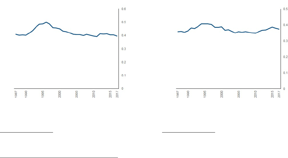
How much might reasonable people have expected real rents to grow? Figures 9 and 10

suggest a clear answer. They show that average rents have been stable relative to incomes –

measured either as relative to real average household income (the income measure used in Figure

2) or rents relative to average earnings (as used in the house price to income ratio shown in Figure

3).

4

Figure 9: Average annual rents as a propor-

tion of average disposable household income

a

a

Data on rents is imputed from the Bank of England’s Financial

Policy Committee’s core indicator on rental yields and average UK

house prices from the ONS UK House Price Index.

Figure 10: Average annual rents as a propor-

tion of average gross earnings

a

a

Data on rents is imputed from the Bank of England’s Financial

Policy Committee’s core indicator on rental yields and average UK

house prices from the ONS UK House Price Index.

4

This is broadly consistent with other data. The UK Housing Review 2019 data includes a series of all private

rents as a ratio to earnings. The series for the four home nations are not provided across consistent time periods,

but they indicate that the ratio has been relatively consistent over time (albeit, the share is lower in absolute terms

for the UK as whole). Joyce, Mitchell and Norris Keiller (2017) consider the median weekly rents and incomes of

private-renting households in Britain (excluding London), and show that whilst there was an uptick in the ratio

between 1994 and 1999, from 1999-2015 the two measures seem to move in parallel.

11

Thus a rational expectation would plausibly have been that average real rents would grow at

around the rate of real incomes. This means (conditional on the assumption that, at each point

in time, the risk-free rate, property ownership taxes, maintenance and the risk premium were

expected to be the same for all future periods), house prices would have been expected to grow

in line with average future real incomes. Furthermore, a reasonable anticipation of average future

real income growth might plausibly have changed rather little over time.

This set of assumptions has the following implication: as the risk-free rate, R

t

, fell (at every

point in a way that was not anticipated, not expected to be reversed but also not expected to be

followed by further falls) house prices would rise more sharply than had previously been expected

and rental yields would fall in a way that followed the safe real return lower.

This is consistent with what has happened in the UK. Figure 11 suggests that rental yields

have indeed fallen in line with index-linked yields. The gap – or ‘wedge’ – between the two

has averaged 6.4%. Equation 4 shows that this wedge should be equal to the average value of

δ

t

+ PO

t

− E[ρ

t

] + RP

t

.

Figure 11: Comparison of the rental yield to the 10 year index-linked gilt yields

Verifying our estimate of the model parameters

Is it plausible that the average cost of maintaining a property, paying the necessary taxes and the

risk premium - net of expected real capital gains - could come to around 6%, as implied by Figure

11?

12

Consider each of the components:

• The average annual cost of overall maintenance of a residential property is plausibly

around 2% of the value of the house.

5

This estimate is less realistic at the extremes of the

housing market (with the cheapest of houses potentially requiring proportionately rather

more in maintenance costs and the more expensive houses requiring less). If we add an

estimate of insurance costs, an overall maintenance and depreciation charge of the order of

2%-3% of property value is plausible.

• Over the time horizon considered by this paper, there have been two notable developments

in the tax treatment of property ownership. First, stamp duty on land and property

has become a signiﬁcantly more important tax, with a number of reforms to its application

across the period. This includes moving from applying a single rate of tax on the entire

property price (a ‘slab’ basis), to applying diﬀerent tax rates to portions of a property price

(a ‘slice’ basis, akin to income tax). Moreover, stamp duty land tax has been updated to

advance diﬀerent policy aims – including encouraging ﬁrst time buyers. As at Q1 2019, the

rate of stamp duty due on a residential property transaction depended on, for example, the

price of the property, the type of borrower (ﬁrst time buyers have a limited exemption),

and whether the purchaser holds existing properties. In 1998, ONS data indicates nominal

stamp duty (land and housing) tax receipts of £2.7bn, including commercial receipts –

compared to £12.9bn in receipts for 2018.

6

This far outpaces nominal growth in average

residential housing values, which have tripled over the same period. But stamp duty is a

very small amount of the overall value of housing stock – Savills estimate the total value

of residential housing at £7.29tn in 2018, indicating annual stamp duty receipts (including

commercial receipts) accounted for 0.18% of housing values (2019). HMRC data on the

breakdown of stamp duty receipts by commercial and residential properties indicate that

residential receipts comprise 60%-75% of total receipts across the period 2007-2018.

7

This

provides a proxy for the upper limit of an estimate for residential stamp duty receipts –

5

There is a good deal of evidence on the depreciation of residential structures: Fraumeni (1997) ﬁnds a depreci-

ation rate of between 1.5-3% each year; Van Nieuwerburgh and Weill (2010) simulate house price dispersion using

a depreciation rate of 1.6%; Harding, Rosenthal and Sirmans (2007) suggest depreciation net of maintenance is

2.5%.

6

ONS series MM9F, current receipts from taxes on production – stamp duty, land and housing.

13

0.13% of residential property values. At the same time, mortgage interest relief for owner

occupiers has become obsolete over the period.

8

The cost of mortgage interest relief peaked

in 1990/91, at £7.7bn in nominal terms; it was abolished in full by 2000. Stamp duty and

mortgage interest relief are, individually, relatively small compared to the aggregate value

of residential property.

9

• Measures of the housing risk premium, RP , are a challenge to pin down. Jorda et al

(2017) show that real returns on housing over the very long term are comparable to those of

equities. If the return on houses were also perceived as being as risky as that of a diversiﬁed

portfolio of equities the premium might be 4-6% per annum. They show that aggregate house

price volatility is signiﬁcantly smaller than is equity return variability, however, the price

of individual homes is far more volatile than the return on a diversiﬁed portfolio of equites.

(Case et al. (2005) estimated that it was twice as volatile for the US.) Even so houses are

likely seen as somewhat less risky than equities – in part because, even if their sensitivity

in price to aggregate economic factors is likely to be high, they help hedge against future

rises in house values and rents. For a borrower one additional element of the risk premium

is the mortgage rate spread to the risk-free rate. This has shown signiﬁcant variability from

year to year but no obvious trend. New mortgages at the highest loan to values have high

spreads to the risk-free rate. Across the period 1997-2018, the average mortgage spread on

new loans relative to a reference rate was around 150bps (see Figure 12). But relative to

Bank Rate, interest rates on new variable rate mortgages in the UK over the twenty year

period 1996-2016 ﬂuctuated between 1% and 2%. Overall a mortgage spread of 1-2% on the

stock of mortgages looks plausible and a ﬁgure of 2-3% for the risk premium on housing (i.e.

around half of that of equities). In total, the composite term, RP

t

, (a spread to the safe

rate) might be 3-5%.

We argued above that expected capital gains reﬂect the expected growth in rents, which is

closely linked to the expected growth in incomes. Average growth in real disposable income per

7

Based on stamp duty land tax transactions of £40,000 or more.

8

HMRC data on mortgage interest relief is available on the National Archives. See, for example, here: https:

//webarchive.nationalarchives.gov.uk/20121106040152/http://www.hmrc.gov.uk/stats/mir/menu.htm

9

But they have not been constant. Over the relevant time horizon, homeowners both faced increasingly higher

taxes on purchasing property and decreasing capacity to oﬀset interest on their mortgage from their personal tax

bill. In our ﬁnal results, we accommodate for the change in property ownership tax and beneﬁts in the long run.

14

Figure 12: Spread of residential mortgage quoted rates to the risk-free rate (bps)

10

capita between 1983 and 2018 is 1.4% (adjusted for RPI) - factoring in growth in household

numbers would take aggregate growth in real household disposable income up to around 1.8%.)

Adding these up, a plausible range for δ

t

+ P O

t

− E[ρ

t

] + RP

t

is around 4-6%, slightly below

the average gap of just over 6% shown in Figure 10, though not obviously inconsistent with it.

III The drivers of house prices

Allowing for a long-run supply adjustment

We begin by considering the immediate (short-run) eﬀect of unanticipated changes in real interest

rates. In the short run the stock of housing is ﬁxed, so equilibrium requires that house prices shift

such that overall demand for housing (from owner-occupiers and renters) is unchanged.

Taking logarithms of equation 3, we have:

ln(P

H

t

) = ln(RR

t

) − ln(R

t

+ δ

t

+ PO

t

− E[ρ

t

] + RP

t

) (6)

If rents and user costs do not change after an unanticipated shift in real interest rates (that

is not expected to be reversed) then demand for owner-occupied or rented property would be

unchanged - and with unchanged supply that would constitute the new (short-run) equilibrium.

Equations 1 and 6 imply that, with unchanged rent and in order to keep the user cost of

housing constant:

∆ln(P

H

t

) = −∆ln(R

t

+ δ

t

+ PO

t

− E[ρ

t

] + RP

t

) (7)

15

In evaluating the right hand side of Equation 7, the only component that would change when

real interest rates shift is the direct eﬀect of a move in the risk-free interest rate (R

t

) - provided

that people expect future real interest rates and other components of cost to be then unchanged,

and anticipate rents to keep rising in line with incomes (whose average rate of growth is insensitive

to shifts in medium-term real rates). In this case there would be no shift expectations of the change

in future real house prices (so that E[ρ

t

] - the expected capital gain - does not change). Current

house prices do all the adjustment.

Over a longer horizon, the rise in prices caused by an unanticipated fall in real yields might

generate some extra housing supply. Factoring this in would potentially make inconsistent the

assumption that in future prices and rents rise in line with incomes only. All the evidence suggests

that housing supply in the UK is not very responsive to price, but any supply response would

make the longer term impact of unanticipated falls in real interest rates somewhat less than the

short-run response. We now explore how signiﬁcant this eﬀect could be, and whether long-run

and short-run price changes could be signiﬁcantly diﬀerent.

In equilibrium the change in housing supply (H

s

) must match the change in housing demand

(H

D

). The relevant measure of cost for the demand side is the user cost. From Equation 1:

∆ln(UCH

t

) = ∆ln(P

H

t

) + ∆ln(R

t

+ δ

t

+ PO

t

− E[ρ

t

] + RP

t

) (8)

Demand will also change as a result of income changes – which we assume drive changes in

both the demand for owner occupied housing and rental housing (with an equal income elasticity

of demand of 

y

).

The long-run percentage change in supply (

˙

H

S

) and demand (

˙

H

D

) for housing are given,

respectively, as:

˙

H

S

= φ + 

s

· ∆ln(P

H

t

) (9)

and

˙

H

D

= 

y

· g

y

+ 

d

[∆ln(P

H

t

) + ∆ln(R

t

+ δ

t

+ PO

t

− E[ρ

t

] + RP

t

)] (10)

where 

s

is the elasticity of supply of the housing stock with respect to price; 

d

< 0 is the

elasticity of demand with respect to the user cost; 

y

is the income elasticity of demand for housing

and the change in aggregate log incomes is denoted by g

y

. (Since we focus on aggregate demand

16

for housing it is the change in aggregate disposable income – and not in average household real

disposable income – that is relevant.) φ is a constant representing that part of the rise in the stock

of housing independent of house prices. We shall assume that government policy is for the supply

of new homes (at unchanged real house prices) to match a fraction of extra demand. This implies

that φ = α(

y

g

y

), where α is the fraction of extra demand coming from rising incomes that can

be matched by supply.

Setting these two expressions (in Equations 9 and 10) equal to each other implies:

∆ln(P

H

t

) =



y

(1 − α)



s

− 

d

˙g

y

+



d



s

− 

d

˙

ln(R

t

+ δ

t

+ PO

t

− E[ρ

t

] + RP

t

) (11)

Comparing Equation 8 to Equation 11 shows that the diﬀerence between the short-run and

long-run change in house prices is that in the longer term changes in income matter and the

reaction to an unexpected change in real rates that is nonetheless expected to be permanent is



d



s

−

d

. This will be less than -1 if (but only if) 

s

> 0.

Incorporating housing elasticities into our model

The value of the price elasticity of supply of the stock of housing is central to the question of

whether long-run changes in house prices diﬀer substantially from short-run changes. Estimates

of this price elasticity (of the supply of the stock of housing) in the UK are relatively low – often

virtually indistinguishable from zero. Meen (2005) suggests that since the 1990s, the regional

supply elasticities in the UK have been very low – he estimates the long-run housing stock supply

elasticity for England is insigniﬁcantly diﬀerent from zero. Some papers look speciﬁcally at the

supply elasticity of new housing investment: e.g. Swank et al (2002) report a price elasticity of

supply for new housing of 0.45; OECD (2011) suggest the long-run price elasticity of supply of

housing investment for the UK is around 0.4. Since the stock of housing is considerably larger

than the level of new housing (i.e. investment) the elasticity of the stock, which is the relevant

variable for house prices, is a small fraction of 0.4. If the ﬂow of investment in a year is 1% of the

stock and the ﬂow elasticity is 0.4, then the short-run stock elasticity would be 0.004.

In recent years in England, house building has barely reached 200,000, compared to an existing

housing stock of around 22 million residential properties. So building is just under 1% of the stock

of housing. Applying a price elasticity of new building volumes of 0.4 to a 1% increase in house

prices amounts to just 800 more houses built – even across a 20 year horizon, that is a mere

17

16,000 new houses built, or slightly under 0.0008 of the existing stock. This is equivalent to a

stock elasticity after 20 years of 0.08 - the value we use in the remainder of this paper. At such a

low stock elasticity, people would be rational to believe that the amount of housing is eﬀectively

unchanged by house price changes.

Very low price elasticities of the stock of housing are implied by the sluggish response of

housebuilding to a long period of high and rising house prices. There is little evidence to suggest

that the provision of housing services per capita has increased in the long run. Whilst crude

measures of the number of properties per capita have increased, this aggregate statistic masks two

key underlying trends: the greater building of ﬂats rather than houses, and the smaller size of new

builds. The English Housing Survey 2016

11

stock condition data suggests the prevalence of ﬂats

(converted or purpose built) in the overall stock has increased from 19% in 1996 to 21% in 2016.

Williams (2009) ﬁnds that new houses built in the UK were smaller than the existing stock –

average stock size was 87m

2

compared to a new build size of 83m

2

. Estimates provided by the

Royal Institute of British Architects and also by companies involved in new-build construction

indicate that rooms are smaller in new builds, with many properties not meeting minimum space

standards.

12

And Morgan and Cruickshank (2014) connect the small, and declining, house size of

UK homes with under-occupation of homes. Estimates of the price elasticity of demand are

typically much larger (in absolute magnitude) than the elasticity of supply, but are well short of

unity. Muellbauer and Murphy (1997) estimate the price elasticity at -0.52. Other estimates of

the price elasticity are slightly greater at between -0.5 and -0.8; see, for example Ermisch et al.

(1996) who put the range at between -0.5 and -0.8, or Rognlie (2016) who ﬁnds a slightly larger

range for the elasticity – between -0.4 and -0.8.

The income elasticity of demand tends to vary by methodology. Malpezzi and Wachter

(2012) suggest that micro-studies generate estimates in the 0.5-0.8 range, whilst aggregate studies

tend to produce elasticities closer to unity, as they capture the long run dimension of behaviour.

Muellbauer and Murphy (1997) estimate an income elasticity of housing demand of 1.32, and Meen

and Andrew (1998) estimate an income elasticity of 1.27.

Plausible values of the three key elasticities might therefore be:



s

= 0.08

11

The English Housing Survey 2016 report and data is available here: https://www.gov.uk/government/

statistics/english-housing-survey-2016-stock-condition

12

See Royal Institute of British Architects (2015) and LBC Warranty (2019)

18



d

= −0.6



y

= 1.3

With an income elasticity of demand of 1.3, real disposable income growth for the household

sector in aggregate of around 1.75%, and housing building growing the stock by not even 1%, α

(the fraction of extra demand coming from rising incomes) is at most around 0.5.

Plugging these values into Equation 8 generates a long-run process for house price changes:

∆ln(P

H

t

) =

1.3(1 − 0.5)

0.08 − (−0.6)

· g

y

+

−0.6

0.08 − (−0.6)

· ∆ln(R

t

+ δ

t

+ PO

t

− E[ρ

t

] + RP

t

) (12)

which is approximately equal to:

∆ln(P

H

t

) = g

y

− 0.9 · ∆ln(R

t

+ δ

t

+ PO

t

− E[ρ

t

] + RP

t

) (13)

This would imply that in the long run house prices rise in line with incomes less around 90%

of the change in ln(R

t

+ δ

t

+ PO

t

− E[ρ

t

] + RP

t

)].

Changes in ln[(R

t

+ δ

t

+ P O

t

− E[ρ

t

] + RP

t

)] are dominated by the change in R

t

, the risk-free

rate, which we have argued are unanticipated. The long-run impact of changes in real interest rates

we estimate at about 0.9 times as large as the short-run impact, but this is based on an assumed

price elasticity of the stock of housing as high as 0.08 – a ﬁgure only likely to be achieved around

20 years after an initial rise in house prices. We conclude that it would be reasonable for anyone

to essentially assume that the short-run and long-run impact of a change in real interest rates that

is expected to be permanent is eﬀectively the same over any plausible investment horizon.

IV Accounting for three decades of real house price growth

Equations 7 and 13 show the short-run and long-run drivers of house prices. We use those relations

to estimate how much income growth and changes in real interest rates – both fundamental factors

– might have contributed to the growth in house prices.

13

Figure 11 suggests that the average value for δ +P O − E[ρ] +RP between 1987 and 2018 Q3 is

around 6.4%. If we assume that all these components are at their average value and that the real

gilt yield falls by 1 percentage point from an initial value of 0 then R

t

+ δ

t

+ P O

t

− E[ρ

t

] + RP

t

falls to 5.4%. In the short-run income growth is unchanged, and so a 1 percentage point decrease

13

All series showed in this section are adjusted for RPI. In terms of CPI, growth would be approximately 1%

higher per year.

19

in real gilt yields implies a short-run change in log house prices of +0.169; as a percentage this is

18.4%.

Table 1 computes the eﬀect on house prices of changes in the safe real rate of interest between

1985 and 2018. It assumes the average wedge between the real gilt yield and the overall percentage

user cost of housing of 6.4% applies in all periods.

The table suggests that, in the absence of any supply response, structural changes in the user

cost of housing from declines in real interest rates resulted in a 126% increase in real house prices.

Over this period there is some evidence of a slight net increase in mortgage spreads of perhaps

0.2% or so; if we accounted for that, the impact of interest rate changes on real house prices would

be a bit lower at about 115%.

In December 2018, the real yield on a 10 year index-linked gilt was -2%. A 1 percentage point

increase in gilt yields (to -1%, which is around the value observed in early 2016) that was assumed

to be persistent would be associated with a real house price fall of approximately 18%, arising

across a long period. Were real gilt yields to rise to 0% (levels last seen around 2011), this would

imply a 31% fall in house prices.

Now we factor in a supply response and also allow for some changes in taxes over time.

Table 2 shows that factoring in a change in supply induced by higher house prices somewhat

dampens the impact of a change in real interest rates. We also account for the impact of changes

in the tax system for property ownership – namely, the increasing importance of stamp duty and

the declining importance of mortgage interest relief.

14

As the consequence of changes in taxation,

previously captured within the wedge term, are allowed to vary, the term moves from 6.4% to

just under 6.5%. These tax changes oﬀset a small part of the impact of falling real gilt yields –

reducing the overall impact of all factors besides income growth to about 90%; the pure gilt yield

impact on its own is about 108%. We caveat that our analysis of the changes in taxation over the

period is likely to overstate the change - we do not have data on stamp duty for the beginning

of the period, and due to the volatility of the series, we do not attempt to impute values. This

means the level of housing taxation we assume at the beginning of the period is lower than it

would actually have been, because it does not incorporate stamp duty.

14

This will be an overestimate due to data limitations - data on the land and housing stamp duty receipts is not

available as far back as 1985, and volatility in annual receipts makes generating a plausible back series challenging,

so no stamp duties are attributed to 1985.

20

The tables also show that, across shorter periods within the three decades we are exploring, the

relationship breaks down. This implies that changes in the real risk-free rate play the dominant role

in driving house prices only over the longer term. In the short-term, other factors are more strongly

associated with changes in UK house prices. For example, we noted in Section II that lack of credit

availability does not undermine the model’s key assumptions for the long-term relationship. In the

short-run, however, it is plausible for credit conditions to aﬀect house prices and for this to be a

very relevant factor in the pre-crisis and post-crisis periods. Consider the case of a negative shock

to credit availability: some people are forced into renting though would ideally like to purchase

a home (’reluctant renters’). The housing market clears: properties that the reluctant renters

would have purchased are instead purchased by landlords. This has consequences for rents - both

anticipated and actual - particularly if reluctant renters go on to rent smaller properties (i.e. fewer

housing services) then they might otherwise have purchased.

21

Table 1: The eﬀect of the decline in the risk-free rate on house prices - no supply response

Period

Change in gilt yields across period

(percentage points)

Implied eﬀect on house prices of

change in gilt yields

(100 x delta log - see Equation 6)

Implied change in real house prices

(per cent)

1985-2018 -5.6 81.7 126.4%

1985-2008 -2.0 22.2 24.8%

2008-2018 -3.6 59.5 81.4%

Table 2: The eﬀect of the decline in the risk-free rate on house prices - allowing for a supply response

Period

Growth in house prices

due to changes in gilt

yields

(per cent)

Growth in house

prices due to

tax changes

(per cent)

Growth in house prices

due to rising aggregate

real income

(per cent)

Combined: growth in house prices

due to falling gilt yields, tax

changes, and real incomes

(per cent)

Observed growth in

real house prices

(per cent)

1985-2018 107.7% -15.1% 80.4% 173.0% 156.1%

1985-2008 22.0% -7.1% 73.0% 87.8% 134.9%

2008-2018 70.3% -2.6% 4.3% 72.0% 9.1%

22

Rising incomes, falling real interest rates and changes in tax treatment account for slightly

more than the overall rise in real house prices over the past 33 years (173% versus an outturn

of 156%). There is one additional cost not allowed for here, which plausibly accounts for the

slight over-prediction of house price growth in the results – there has been a slight increase in

the mortgage spreads to the risk-free rate. Some evidence for this increase is provided above (see

Figure 11), though we note that this concerns the ﬂow, rather than the stock. We estimate that

the net eﬀect across the period might be in the region of an increase in costs of 20-30bps. This

would generate expected growth in house prices due to incomes rising, tax changes, gilt yields

falling and a small increase in mortgage spreads of between 161% and 164% - not too far oﬀ the

observed growth in national house prices.

Overall, therefore, the sustained decline in real interest rates over the past 35 years would have

accounted for all of the doubling in house prices relative to disposable incomes.

As was noted at the outset, this paper focuses on the national housing picture. We have

not oﬀered an explanation of regional diﬀerences in the trajectory of house prices. Such regional

diﬀerences are large. They reﬂect a host of factors amongst which are: diﬀerences in the supply

elasticities of housing in more and less densely populated regions; substantial changes in the pattern

of employment and the decline and rise of diﬀerent industries which are regionally concentrated;

changes over time in the importance of proximity to other ﬁrms and workers to productivity

(agglomeration eﬀects); and variability in the quality of transport infrastructure.

An international comparison

The 30 year decline in index-linked gilt yields has been a global phenomenon: Figure 7 shows how

a ‘world’ interest rate – derived from the G7 excluding Italy – has changed since 1985. Whilst this

paper concerns the eﬀect that the decline in the 10 year index-linked yield in the UK has had on

UK house prices, the global decline suggests that a corresponding eﬀect should be experienced in

other countries.

In the brief, illustrative analysis that follows, we consider what the model might predict were

the UK to have elasticities of supply, demand, and income, closer to those estimated for other

developed countries, and if the fall in the risk-free rate were smaller (and therefore closer to that

observed in the other G7 countries).

In particular:

23

• We double the stock elasticity of housing supply. The estimate of this elasticity above,

0.08, is based on a ﬂow elasticity of housing supply of 0.4 – see OECD (2011). Doubling

the stock elasticity, to 0.16, would be consistent with (but still short of) the underlying ﬂow

elasticities of Canada, Japan and Denmark (yet remains considerably smaller than the US).

• We apply an income elasticity of demand of 0.7. Whilst the main analysis assumed

an elasticity of 1.3 based on UK literature, Albouy, Ehrlich and Yiu (2016) estimate that

the US income elasticity of demand is around 0.7.

• We maintain the price elasticity of demand at -0.6. Albouy, Ehrilich and Yiu (2016)

estimate the price elasticity of housing demand for the US at -0.7; a literature review of the

same statistic produced for Canada’s housing department suggested a range of -0.5 to -1.0

(Skaburskis, 1999).

• We set the decline in gilt yields to around 4pp. This is consistent with the US

experience set out in Figure 8; the US ends the period at a higher risk-free rate than the

world risk-free rate (which in turn is higher than the UK end-2018 rate).

Inserting these revised ﬁgures into Equation 11 produces:

∆ln(P

H

t

) = 0.74 · g

y

− 0.79 · ∆ln(R

t

+ δ

t

+ PO

t

− E[ρ

t

] + RP

t

) (14)

This would suggest that, if UK elasticities were closer to values in other developed countries

(i.e. the supply elasticity larger, the income elasticity smaller) and the decline in gilt yields a little

smaller, the model predicts real house price growth would have amounted to 88%, (of which, 55%

would have been due to income growth, and 40% due to the decline in the risk-free rate – with

a small oﬀsetting eﬀect from changes in taxation). This contrasts with the 173% predicted when

UK values are used.

V Concluding remarks

In this paper, we have presented evidence connecting the decline in the real yield on index-linked

gilts, as a proxy for the risk-free rate, to rising house prices and falling rental yields over the long

term. The conclusions are stark – since 1985, the observed decline in index-linked gilt yields and

24

other changes in the cost of home ownership are associated with an increase in house prices of

around 90%; income rises account for about a further rise of 80% - between them these factors

account for all of the observed rise.

This does not mean that other factors are unimportant for short-run ﬂuctuations in prices; the

equilibrium conditions explored here provide an explanation for the long-run trajectory in house

prices. Over shorter horizons house prices will be driven by other factors – such as movements in

mortgage availability, shifts in uncertainty and the ups and down of the business cycle. Over the

longer term one can account for all of the rise in house prices relative to incomes as being due to

persistent declines in real interest rates.

Today global yields on inﬂation-proof government bonds are at a historical low. In the UK,

the 10 year index-linked gilt yield in early 2019 was a little under -2.0%. Were the 35 year trend

to reverse, and gilt yields to rise rather than fall, this research indicates that there would be a very

substantial long-term consequence for real house prices. Our results suggest that a 1% change in

real interest rates that was persistent could move real house prices by just under 20% across many

years.

This calculation illustrates the sensitivity of house prices to changes in interest rates. But it

does not suggest that house prices are likely to move lower. That would only be reasonable if a

reversal of the 30 year downwards trend in safe real interest rates seemed likely. But measures

of real interest rates in the UK and other developed countries show little sign of mean revision

(see Figures 6, 7 and 8). We also noted that forward rates consistently move in line with spot

rates implying that what is priced into bond markets has consistently been that the best estimate

of yields in the future is the current rate. That is consistent with a random walk model of real

yields and not with mean reversion. Nor do explanations of the current low level of real interest

rates (be they based on secular stagnation hypothesis or a savings glut story) give much reason

to anticipate a reversion to higher real rates.

25

VI Appendix: Household optimisation, the user cost and

rents

We assume that agents (indexed by i) derive utility from the consumption of goods, denoted C,

and of housing services. Housing services are assumed to be proportional to the (quality adjusted)

size of the house (H

i

) - which is the number of units of housing the household enjoys. We can

express utility as a function of consumption of goods and of the size of the house in which the

agent lives (either rented or owned). Preferences over these goods at a given time t is described

by a utility function which shows the ﬂow of utility for agent i at time t (denoted Q

it

)

Q

it

= U [C

it

, H

it

] (15)

Lifetime utility (W

i

) is the discounted sum of per period utility

W

i

=

T

X

t=0

Q

it

/(1 + η)

t

(16)

T is the planning horizon; η is the discount factor (rate of time preference).

Assume initially that the household can borrow enough with a mortgage (of size M), in con-

junction with accumulated net ﬁnancial wealth S, to buy a house which generates housing services.

Assume also that the real return on ﬁnancial assets and the real interest rate on mortgage debt

are both equal to r

t

. This rate r

t

is not the safe rate (which we denote R

t

) because the average

asset that households hold in their portfolio of non-housing wealth (S

it

), as well as mortgage debt,

are both assumed to be less secure than is the return on a truly riskless real asset, such as an

inﬂation indexed government bond. The risk premium on S and M is RP

t

so that r

t

= R

t

+ RP

t

.

The consumption good is the numeraire. The period to period budget constraint is:

C

it

= Y

it

+ (1 + r

t

)S

it−1

− S

it

− (1 + r

t

)M

it−1

+ M

it

− P

t

(H

it

− (1 − δ)H

it−1

) − P

t

H

it

(P O

t

)

subject to the constraints:

S

it

 0

M

it

 0

S

iT

+ P

T

H

iT

− M

iT

 0

26

where:

Y

it

is labour income;

P

t

is the price of a unit of housing at time t in terms of consumer goods;

P O

t

is the tax rate on housing for owners of property, and P

t

H

it

(P O

t

) is total tax paid; and

δ is the cost of home maintenance (to oﬀset depreciation) plus other home ownership costs

that are related to the size of the property, such as insurance.

The ﬁrst order conditions for optimal consumption of goods and of housing services are:

dU

i

/dC

it

= [(1 + r

t

)/(1 + η)]dU

i

/dC

it+1

(17)

dU

i

/dH

it

= dU

i

/dC

it

[P

t

{r

t

+ δ + P O

t

− ρ

t

}] (18)

where ρ

t

is the rate of change of house prices (i.e. the rate of real capital gains on housing,

which we assume is untaxed)

The optimising condition (Equation 18) is that the rate of substitution between housing services

and consumer goods, (dU

i

/dH

it

)/(dU

i

/dC

it

), should equal the rate of transformation in cost terms,

P

t

{r

t

+ δ + P O

t

− ρ

t

} , where the latter is the user cost of housing. The user cost is the real cost

of housing services. If we substitute in the relation between the safe rate of interest and the return

on both mortgages and non-housing wealth (that is r

t

= R

t

+ RP

t

) we can write the user cost

(UCH

t

) as:

UCH

t

= P

t

{R

t

+ δ + P O

t

− ρ

t

+ RP

t

} (19)

This is the form of the user cost formula used in the main text.

If there are some households that are indiﬀerent between renting and owning then rent paid

must equal the user cost of housing, a condition we assume holds.

27

VII Bibliography

Albouy, D., Ehrlich, G., Liu, Y., (2016). “Housing demand, cost-of-living inequality, and

the aﬀordability crisis”. NBER Working Paper Series: 01 July 2019. Available from: https:

//www.nber.org/papers/w22816.pdf

Barker, K., (2004). “Review of Housing Supply”. Place of Publication: BBC. [01 February

2019] Available from: http://news.bbc.co.uk/nol/shared/bsp/hi/pdfs/17_03_04_barker_

review.pdf

Case, K., Quigley, J., Shiller, R., (2005). “Comparing Wealth Eﬀects: The Stock Market

versus the Housing Market”. Advances in Macroeconomics 5(1)

Skaburskis, A., (1999). “The eﬀect of development charges on urban form: an econometric

analysis”. Canada Mortgage and Housing Corporation. [1 July 2019] Available here: http://

publications.gc.ca/collections/collection_2017/schl-cmhc/nh18-1-4/NH15-325-1999-eng.

pdf

Ermisch, J.F., Findlay, J., Gibb, K., (1996). “The Price Elasticity of Housing Demand

in Britain: Issues of Sample Selection”. Journal of Housing Economics, 5(1), pp64-86

Fraumeni, B., (1997). “The measurement of depreciation in the US national income product

accounts”. Survey of Current Business 77, 7.23.

Green, R., Malpezzi, S., Mayo, S., Harding, J., Rosenthal, S., and Sirmans, C.,

(2007). “Depreciation of housing capital, maintenance, and house price inﬂation: Estimates from

a repeat sales model”. Journal of Urban Economics 61(2), pp193-217.

Harding, J., Rosenthal, S., and Sirmans, C., (2007). “Depreciation of housing capital,

maintenance, and house price inﬂation: Estimates from a repeat sales model”. Journal of Urban

Economics 61(2), pp193-217.

Jorda, Knoll, Kuvshinov, Schularick and Taylor (2017). “The Rate of Return on

Everything”. NBER Discussion Paper 24112, December.

28

Joyce, R., Mitchell, M., Norris Keiller, A., (2017). “The cost of housing for low-income

renters. The Institute for Fiscal Studies: 01 July 2019. Available at: https://www.ifs.org.uk/

uploads/publications/comms/R132.pdf

King, M., and Low, D., (2014). “Measuring the “World” Real Interest Rate”. [28 March

2019] Available at: https://www.nber.org/papers/w19887.pdf

Kneuzel, R., and Bjornbak, B., (2008). “The UK Housing Market: Anatomy of a

house price boom”. [29 March 2019]. Available at: http://ec.europa.eu/economy_finance/

publications/pages/publication13282_en.pdf

LBC Warranty (2019). ”What is the average house size in the UK?” [1 June 2019]. Available

at: https://www.labcwarranty.co.uk/blog/are-britain-s-houses-getting-smaller-new-data/

Meen, G., (2005). “On the Economics of the Barker Review of Housing Supply”. [01

February 2019] Available at: https://doi.org/10.1080/02673030500291082

Meen, G., Andrew, M., (1998). ”Modelling Regional House Prices: A Review of the

Literature, prepared for the Department of the Environment, Transport and the Regions”. ISBN:

0 7049 1305 4

Miles, D (1994). ”Housing Financial Markets and the Wider Economy”. John Wiley.

Ministry of Housing, Communities and Local Government, (2018). “House building;

new build dwellings, England: December Quarter 2017”. [02 April 2019] Available at: https://

assets.publishing.service.gov.uk/government/uploads/system/uploads/attachment_data/

file/692680/House_Building_Release_Dec_Qtr_2017.pdf

Malpezzi, S., Wachter, S.M., (2012). “Housing Demand”. International Encyclopedia of

Housing and Home, pp404-407.

Morgan, M., and Cruickshank, H., (2014). “Quantifying the extent of space shortages:

English dwellings”. Building Research and Information, 42(6), pp710-724.

Muellbauer,J., and Murphy, A., (1997). “Booms and Bust in the UK Housing Market”.

The Economic Journal, 107(445), pp1701-1727.

29

National Audit Oﬃce, (2017). “Housing in England: overview”. [11 March 2019] Available

at: https://www.nao.org.uk/wp-content/uploads/2017/01/Housing-in-England-overview.

pdf

OECD (2011). “The Price Responsiveness of Housing Supply in OECD Countries”. [28

March 2019] Available at: https://doi.org/10.1787/5kgk9qhrnn33-en

Peachey, K., (2019). “Typical council tax in England will rise by 4.7% in April”. British

Broadcasting Corporation [online]. 27 March 2019. Available at: https://www.bbc.co.uk/news/

business-47718718

Poterba, J. (1984). “Tax Subsidies to Owner Occupied Housing: An Asset-Market Ap-

proach”. The Quarterly Journal of Economics, 99(4), pp729–752.

Rognlie, M., (2016). “Deciphering the fall and rise in the net capital share: Accumulation

or Scarcity?”. Brookings papers on economic activity, 2015(1), pp1-69.

Royal Institute of British Architects (2015). ”Space standards for homes”. [1 June 2019]

Available at: https://www.architecture.com/-/media/gathercontent/space-standards-for-homes/

additional-documents/homewisereport2015pdf.pdf

Sa, F., (2016). “The Eﬀect of Foreign Investors on Local Housing Markets: Evidence from

the UK”. Accessed 12 March 2019, available at: https://papers.ssrn.com/sol3/papers.cfm?

abstract_id=2877263

Savills, (2019). ”Value of UK housing stock hits record high”. [20 May 2019] Available at:

https://www.savills.co.uk/blog/article/274512/residential-property/value-of-uk-housing-stock-hits-record-high.

aspx

Seely, A., and Keep, M., (2018). “Stamp duty land tax on residential property”. House

of Commons Library Brieﬁng Paper no. 7050. London: House of Commons Library. Available at:

https://researchbriefings.files.parliament.uk/documents/SN07050/SN07050.pdf

Summers, L., and Rachel, L., (2019). “On Falling Neutral Real Rates, Fiscal Policy, and

the Risk of Secular Stagnation”. [28 March 2019] Available at: https://www.brookings.edu/

30

wp-content/uploads/2019/03/On-Falling-Neutral-Real-Rates-Fiscal-Policy-and-the-Risk-of-Secular-Stagnation.

pdf

Swank. J, Kakes, J., Tieman, A., (2002). “The Housing Ladder, Taxation, and Bor-

rowing constraints”. [30 March 2019] Available at: https://econpapers.repec.org/paper/

dnbwormem/688.htm

Van Nieuwerburgh, S., and Weill, P., (2010). “Why has house price dispersion gone

up?”. The Review of Economic Studies, 77(4), pp1567-1606.

Williams, K., (2009). “Space per person in the UK: A Review of densities, trends, ex-

periences and optimum levels”. [20 January 2019] Available at: https://doi.org/10.1016/j.

landusepol.2009.08.024

31